
semilogy — Plot data with a logarithmic y-axis using MATLAB-compatible semilogy call patterns.
semilogy creates line plots like plot and configures the active axes to logarithmic scaling on Y. It follows MATLAB-compatible argument forms, axes targeting, and handle behavior.
Syntax
h = semilogy(Y)
h = semilogy(X, Y)
h = semilogy(args...)
Inputs
| Name | Type | Required | Default | Description |
|---|---|---|---|---|
Y | NumericArray | Yes | — | Y data vector/matrix. |
X | NumericArray | Yes | — | X data vector/matrix. |
args | Any | Variadic | — | Plot-style inputs: optional axes handle, style tokens, and Name/Value pairs. |
Returns
| Name | Type | Description |
|---|---|---|
h | NumericScalar | Line handle. |
Errors
| Identifier | When | Message |
|---|---|---|
RunMat:semilogy:PlotFailed | Underlying plot rendering/parsing fails while building the semilog plot. | semilogy: plot operation failed |
RunMat:semilogy:LogAxisFailed | Applying logarithmic Y-axis mode fails. | semilogy: failed to apply logarithmic axis mode |
How semilogy works
- The returned value is a numeric line handle.
- Only the y-axis is switched to log scale; the x-axis remains linear.
- Y log-mode state is subplot-local and does not leak into other subplot axes.
- Positive y-values are the meaningful domain for a logarithmic y-axis.
Examples
Plot an exponential decay on a logarithmic y-axis
t = linspace(0, 10, 200);
semilogy(t, exp(-t));
Compare multiple decays on the same axes
t = linspace(0, 10, 200);
h1 = semilogy(t, exp(-t));
set(h1, 'DisplayName', 'exp(-t)');
hold on;
h2 = semilogy(t, exp(-0.3*t));
set(h2, 'DisplayName', 'exp(-0.3t)');
legend;
Inspect the y-axis scale after plotting
t = 0:0.1:4;
semilogy(t, exp(t));
ax = gca;
get(ax, 'YScale')
Expected output:
ans =
    'log'
Rendered semilogy example
time = linspace(0, 12, 300);
fast = exp(-0.85*time);
slow = exp(-0.38*time);

h1 = semilogy(time, fast);
set(h1, 'LineWidth', 2, 'DisplayName', 'Fast decay');
hold on;
h2 = semilogy(time, slow, '--');
set(h2, 'LineWidth', 2, 'DisplayName', 'Slow decay');
hold off;
title('Decay Rate Comparison');
xlabel('Time (s)');
ylabel('Normalized response');
legend();
grid on;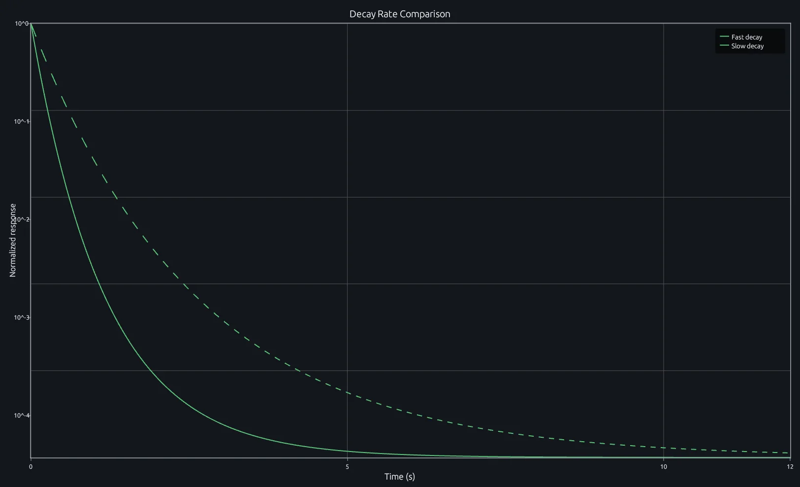
Compare this result with other chart types in the MATLAB Plot Gallery.
Using semilogy with coding agents
Open a RunMat example with live inputs, then ask the agent to explain how semilogy changes the result.
Run a small semilogy example, explain the result, then change one input and compare the output.
FAQ
When is semilogy the right choice over a linear plot?⌄
Whenever the interesting structure lives in multiplicative changes along Y — exponential decay, growth rates, signal attenuation. On a log y-axis, exp(-t) becomes a straight line, which makes decay constants easy to read directly from the slope.
How do I visualize exponential decay and read the time constant?⌄
Plot with semilogy and the decay appears as a straight line. The slope of that line is the decay rate. For exp(-t/tau), the signal drops by a factor of e every tau units along the x-axis.
t = linspace(0, 10, 200);
semilogy(t, exp(-t/3)); % tau = 3
grid on;
What about zero or negative y-values on a log y-axis?⌄
They're excluded from rendering since log of zero or negative numbers is undefined. The data handle still stores them, but only positive y-values produce visible points. If your data crosses zero, consider splitting into positive and negative series or using a linear axis.
Related Plotting functions
2D Charts
area · bar · errorbar · heatmap · hist · histogram · loglog · pie · plot · scatter · semilogx · stairs · stem
Other
addpoints · ancestor · animatedline · axes · barh · caxis · cla · clf · clim · colorcube · colororder · copyobj · daspect · datacursormode · dataTipTextRow · fcontour · figure · fill · fill3 · findobj · fsurf · gobjects · groot · hgload · hgsave · hidden · histogram2 · hold · line · linkaxes · openfig · opengl · pan · parula · patch · plotmatrix · plotyy · polarhistogram · polarplot · polarscatter · print · quiver3 · ribbon · saveas · savefig · sphere · stackedplot · subtitle · suptitle · text · textscatter · textscatter3 · triplot · waitbar · wordcloud · xlabel · xlim · xline · xscale · xtickangle · xtickformat · xticklabels · xticks · ylabel · ylim · yline · yscale · ytickangle · ytickformat · yticklabels · yticks · zlim · zoom
More plotting resources
Open-source implementation
Unlike proprietary runtimes, every RunMat function is open-source. Read exactly how semilogy is executed, line by line, in Rust.
- View the source for semilogy in Rust on GitHub
- Learn how the RunMat runtime works
- Found a bug? Open an issue with a minimal reproduction.
About RunMat
RunMat is an open-source runtime that executes MATLAB-syntax code blazing on any GPU. It is licensed under the Apache 2.0 license.
- RunMat automatically optimizes your math for GPU execution on Apple, Nvidia, and AMD hardware. No code changes needed. Simulations that took hours now take minutes.
- Start running code in seconds. RunMat runs in the browser, on the desktop, or from the CLI. No license server, no IT ticket.