Plot gallery

MATLAB Plot Gallery: Examples with Runnable Code

Browse plots by the relationship you need to show, then open the attached MATLAB-syntax example and replace its sample data. Every image on this page was rendered by RunMat from the code on its card.

If you are deciding between several representations, read how to choose the right MATLAB plot type.

Showing 31 of 31 plot examples

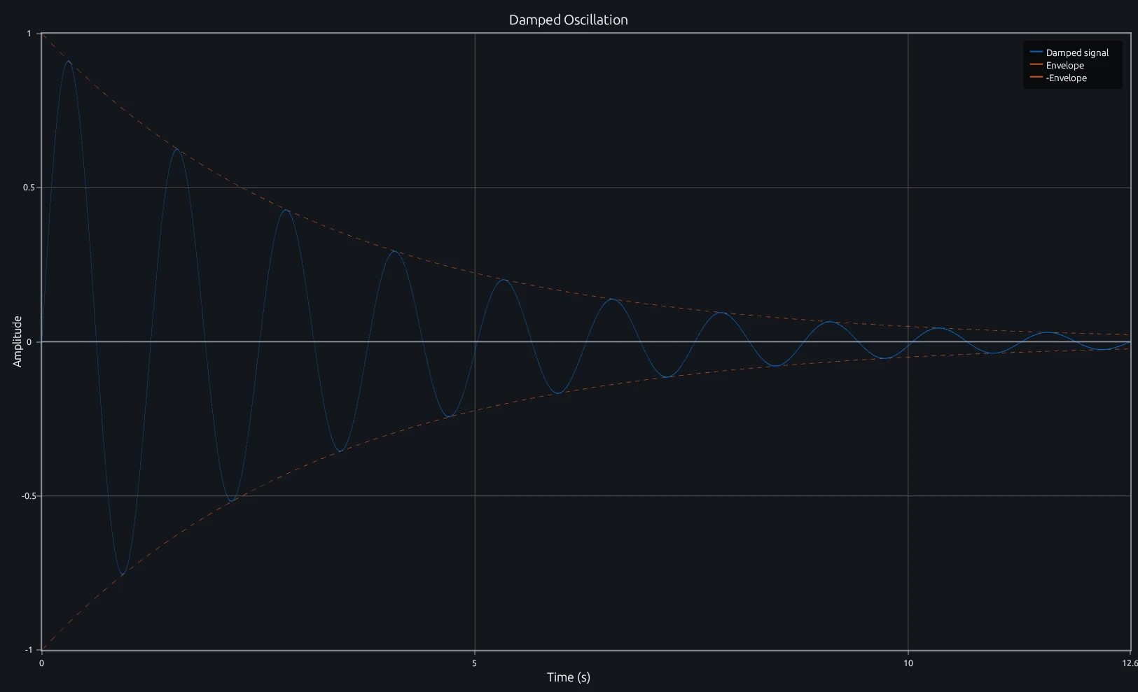
Damped oscillation and its upper and lower envelopes rendered as a MATLAB line plot in RunMat

plot

Trace a damped oscillation—or any response whose point-to-point progression carries meaning.

View MATLAB-syntax code
t = linspace(0, 4*pi, 500);
envelope = exp(-0.3*t);
signal = envelope .* sin(5*t);

h1 = plot(t, signal);
set(h1, 'DisplayName', 'Damped signal', 'LineWidth', 1.5);
hold on;
h2 = plot(t, envelope, '--');
set(h2, 'DisplayName', 'Envelope', 'LineWidth', 1.5, 'Color', [0.85 0.33 0.1]);
h3 = plot(t, -envelope, '--');
set(h3, 'DisplayName', '-Envelope', 'LineWidth', 1.5, 'Color', [0.85 0.33 0.1]);
hold off;

title('Damped Oscillation');
xlabel('Time (s)');
ylabel('Amplitude');
legend();
grid on;
View plot builtin reference
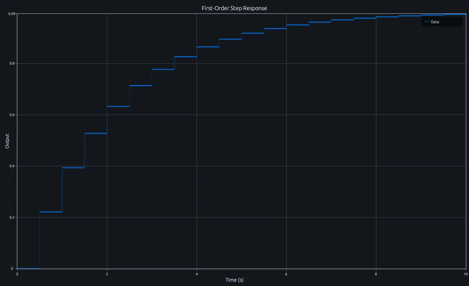
First-order step response rendered as a piecewise-constant MATLAB stair plot in RunMat

stairs

Show a sampled controller output that holds its value until the next update.

View MATLAB-syntax code
t = 0:0.5:10;
y = 1 - exp(-0.5*t);

h = stairs(t, y);
set(h, 'LineWidth', 2);
title('First-Order Step Response');
xlabel('Time (s)');
ylabel('Output');
grid on;
View stairs builtin reference
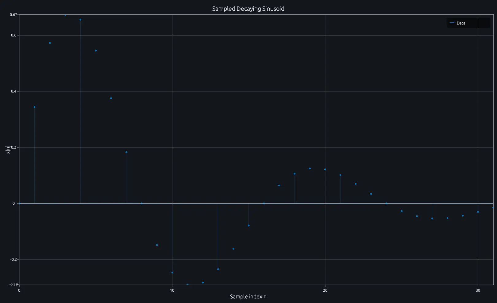
Decaying discrete sinusoid rendered as a MATLAB stem plot in RunMat

stem

Make individual samples and their distance from a shared baseline easy to inspect.

View MATLAB-syntax code
n = 0:31;
x = sin(2*pi*n/16) .* (0.9 .^ n);

stem(n, x);
title('Sampled Decaying Sinusoid');
xlabel('Sample index n');
ylabel('x[n]');
grid on;
View stem builtin reference
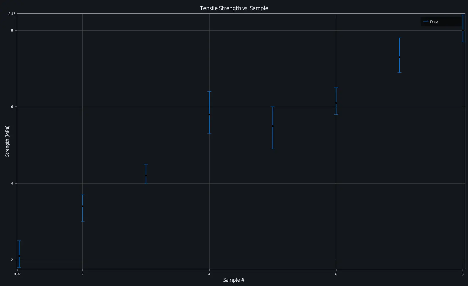
Eight tensile-strength measurements with asymmetric confidence intervals rendered in RunMat

errorbar

Report tensile-test measurements together with their asymmetric uncertainty.

View MATLAB-syntax code
x = 1:8;
y = [2.1 3.4 4.2 5.8 5.5 6.1 7.3 8.0];
neg = [0.3 0.4 0.2 0.5 0.6 0.3 0.4 0.3];
pos = [0.4 0.3 0.3 0.6 0.5 0.4 0.5 0.4];

errorbar(x, y, neg, pos, 'o-', 'LineWidth', 1.5);
title('Tensile Strength vs. Sample');
xlabel('Sample #');
ylabel('Strength (MPa)');
grid on;
View errorbar builtin reference
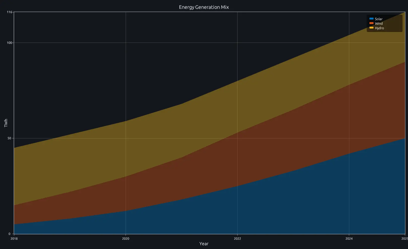
Solar, wind, and hydro generation rendered as a stacked MATLAB area plot in RunMat

area

Show how several generation sources contribute to the total energy supplied over time.

View MATLAB-syntax code
years = 2018:2025;
solar   = [5  8  12 18 25 33 42 50];
wind    = [10 14 18 22 28 32 36 40];
hydro   = [30 30 29 28 27 27 26 26];
mix = [solar; wind; hydro]';

area(years, mix);
title('Energy Generation Mix');
xlabel('Year');
ylabel('TWh');
legend('Solar', 'Wind', 'Hydro');
grid on;
View area builtin reference
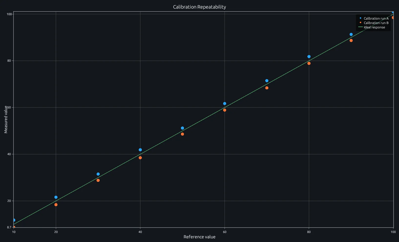
Two calibration runs compared with an ideal response using a MATLAB scatter plot in RunMat

scatter

Compare calibration runs point by point without implying a continuous path between measurements.

View MATLAB-syntax code
reference = 10:10:100;
run_a = [11.8 21.6 31.5 41.9 51.2 61.7 71.5 81.8 91.3 101.0];
run_b = [8.7 18.4 28.8 38.5 48.6 58.9 68.4 78.9 88.7 98.5];

scatter(reference, run_a, 90, [0.15 0.65 1.0], 'filled');
hold on;
scatter(reference, run_b, 90, [1.0 0.45 0.2], 'filled');
plot([10 100], [10 100], '--', 'LineWidth', 1.5);
hold off;
legend('Calibration run A', 'Calibration run B', 'Ideal response');
title('Calibration Repeatability');
xlabel('Reference value');
ylabel('Measured value');
grid on;
View scatter builtin reference
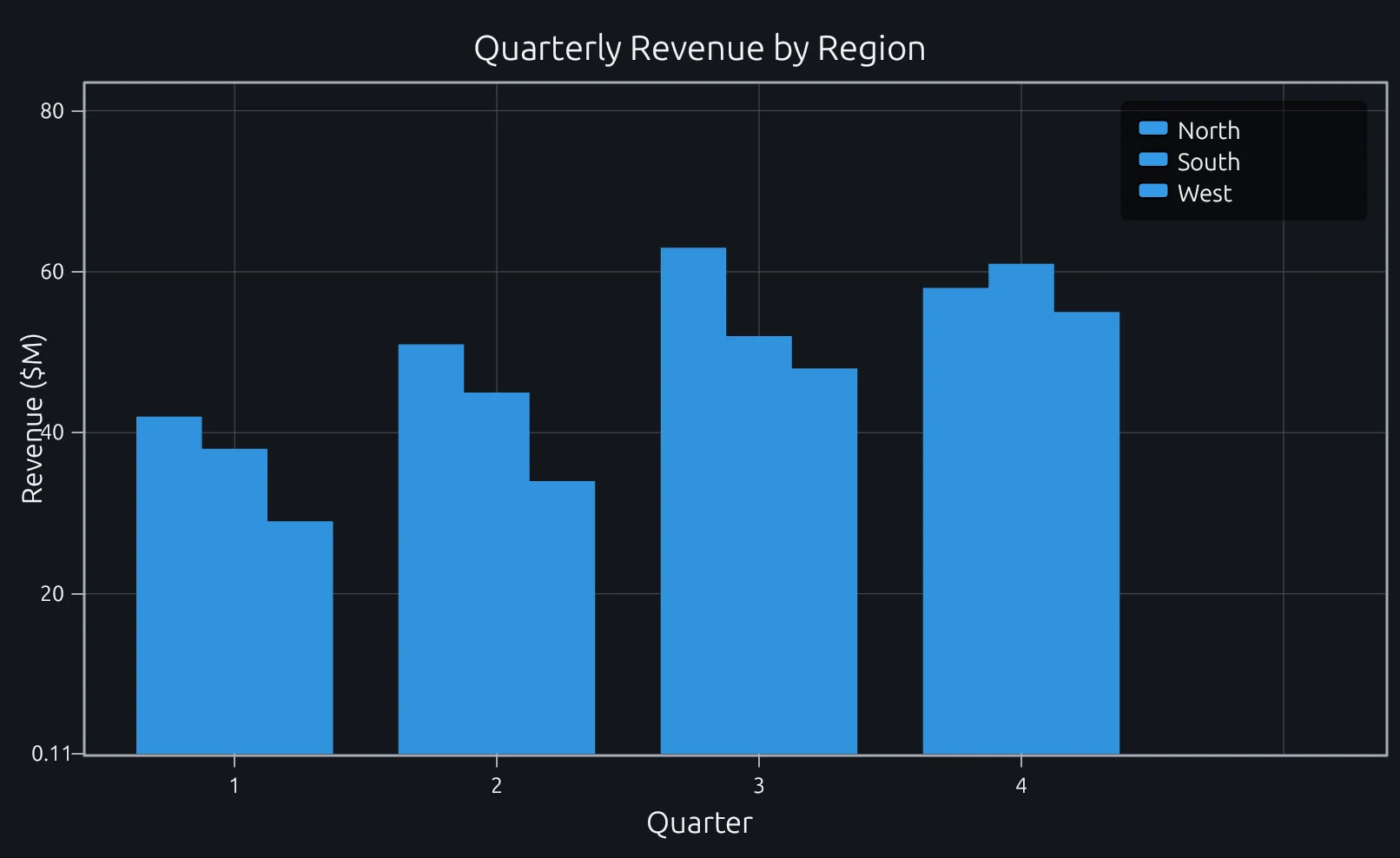
Quarterly revenue for three regions rendered as a grouped MATLAB bar chart in RunMat

bar

Put quarterly results from named regions side by side for a direct comparison.

View MATLAB-syntax code
categories = {'Q1', 'Q2', 'Q3', 'Q4'};
revenue = [42 51 63 58; 38 45 52 61; 29 34 48 55];

bar(revenue');
title('Quarterly Revenue by Region');
xlabel('Quarter');
ylabel('Revenue ($M)');
legend('North', 'South', 'West');
grid on;
View bar builtin reference
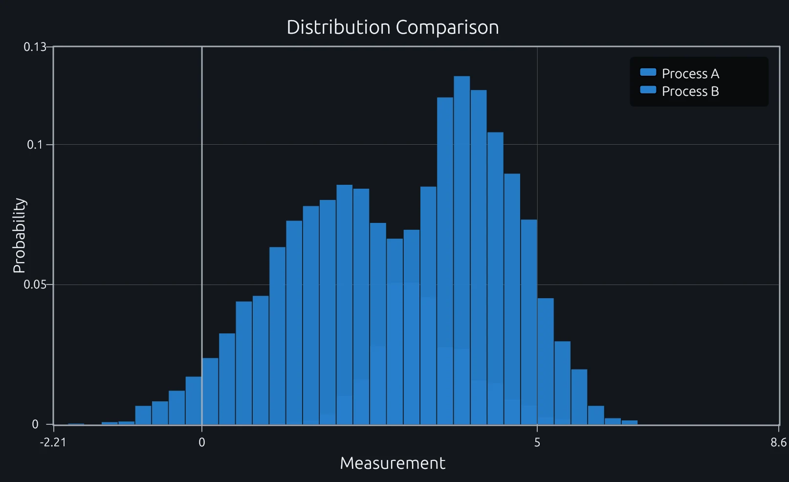
Two process distributions rendered as overlaid probability histograms in RunMat

histogram

Compare the spread, center, and overlap of two sets of repeated measurements.

View MATLAB-syntax code
rng(7);
a = 2 + 1.2*randn(1, 5000);
b = 4 + 0.8*randn(1, 5000);

h1 = histogram(a, 'BinEdges', -2:0.25:8, 'Normalization', 'probability');
set(h1, 'DisplayName', 'Process A');
hold on;
h2 = histogram(b, 'BinEdges', -2:0.25:8, 'Normalization', 'probability');
set(h2, 'DisplayName', 'Process B');
hold off;

title('Distribution Comparison');
xlabel('Measurement');
ylabel('Probability');
legend();
grid on;
View histogram builtin reference
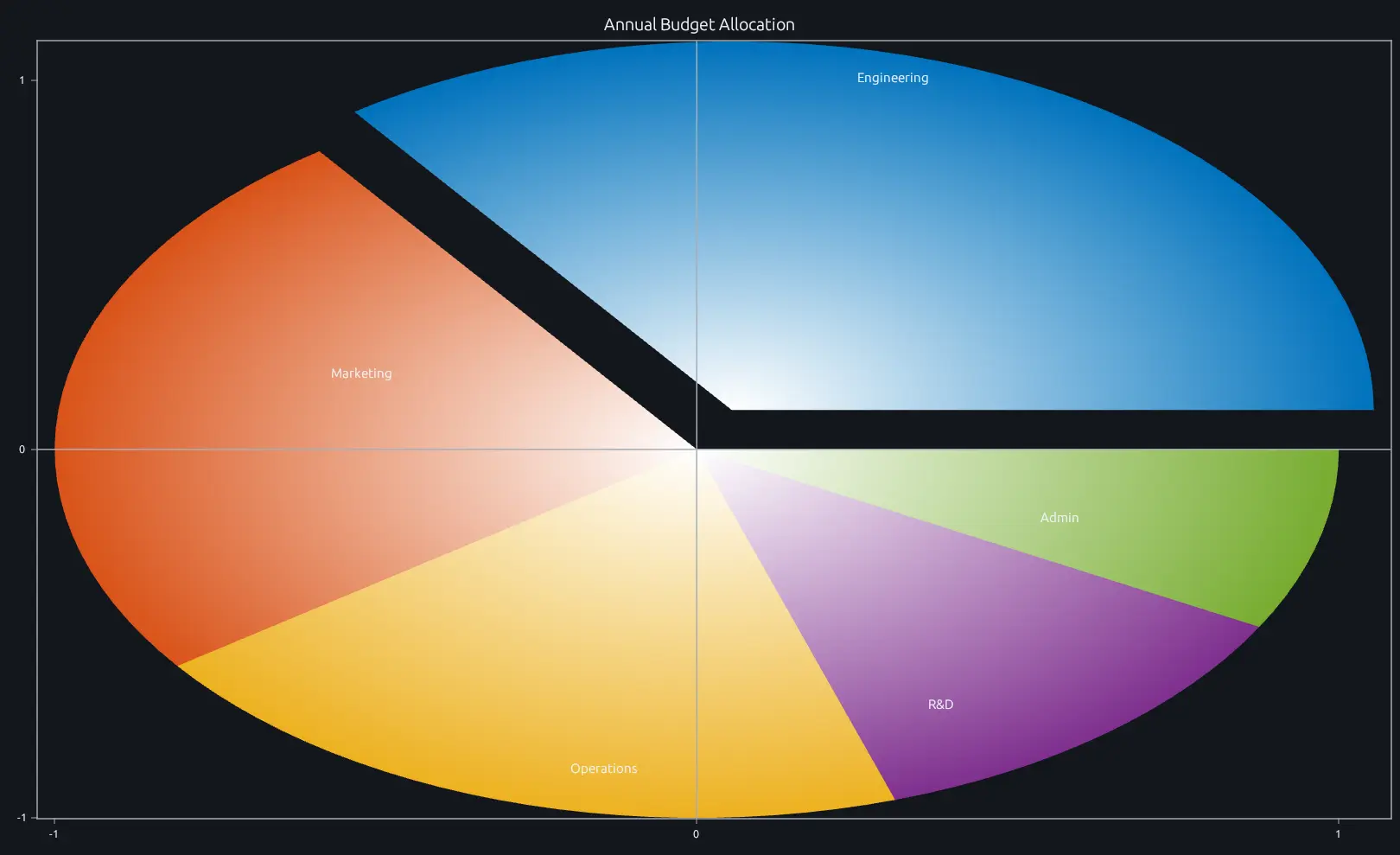
Annual budget allocation rendered as a MATLAB pie chart in RunMat

pie

Summarize a small budget where the share of one fixed total is the main point.

View MATLAB-syntax code
values = [35 25 20 12 8];
labels = {'Engineering', 'Marketing', 'Operations', 'R&D', 'Admin'};
explode = [1 0 0 0 0];

pie(values, explode);
title('Annual Budget Allocation');
legend(labels);
View pie builtin reference
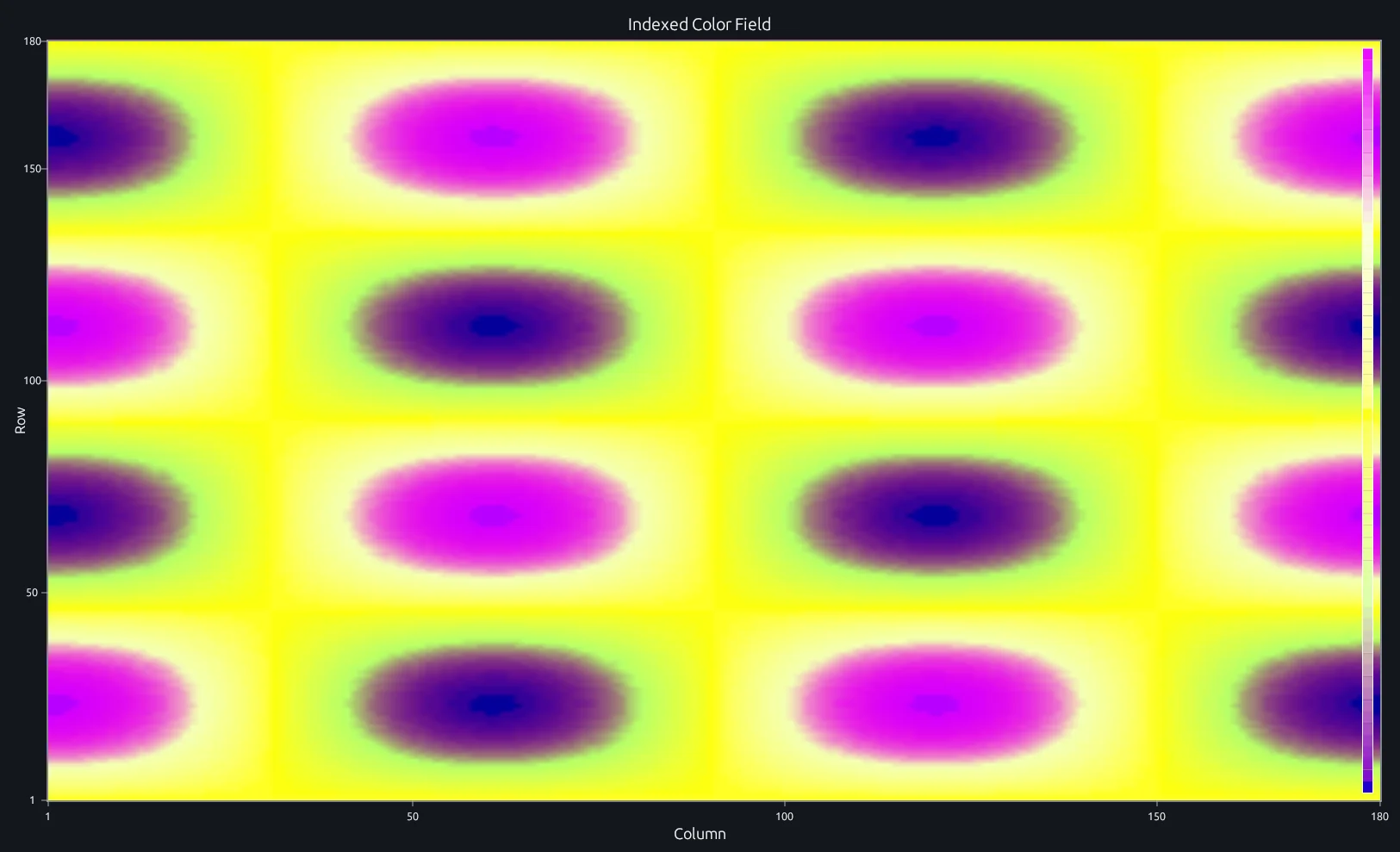
Synthetic indexed color field displayed with the MATLAB image function in RunMat

image

Render a matrix whose values already represent indexed colors or truecolor RGB pixels.

View MATLAB-syntax code
[X, Y] = meshgrid(linspace(0, 1, 180), linspace(0, 1, 180));
pattern = 0.5 + 0.5*sin(4*pi*X).*cos(3*pi*Y);
color_index = round(1 + 63*pattern);

image(color_index);
colormap('turbo');
colorbar;
title('Indexed Color Field');
xlabel('Column');
ylabel('Row');
axis equal;
View image builtin reference
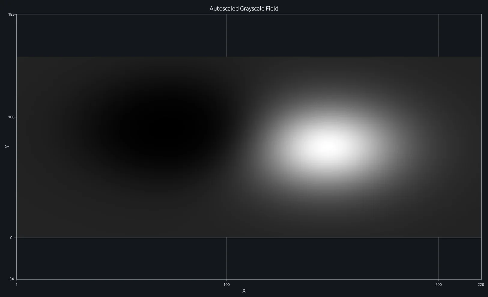
Autoscaled grayscale test field displayed with MATLAB imshow in RunMat

imshow

Inspect grayscale image data with its intensity range mapped cleanly to the display.

View MATLAB-syntax code
[X, Y] = meshgrid(linspace(-3, 3, 220), linspace(-2, 2, 150));
field = exp(-0.8*((X-1).^2 + Y.^2)) - 0.7*exp(-((X+1).^2 + (Y-0.4).^2));

imshow(field, []);
title('Autoscaled Grayscale Field');
View imshow builtin reference
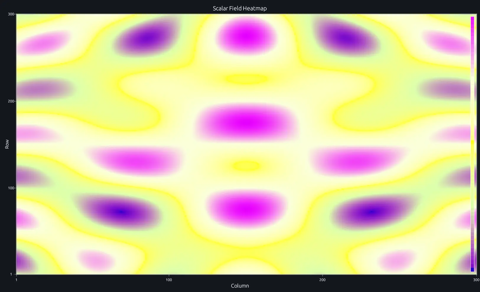
Dense scalar field rendered as a scaled MATLAB matrix image in RunMat

imagesc

Turn a dense scalar field into a color-mapped view so spatial structure is immediately visible.

View MATLAB-syntax code
[X, Y] = meshgrid(linspace(-pi, pi, 300), linspace(-pi, pi, 300));
Z = sin(3*X) .* cos(2*Y) + cos(X.*Y);

imagesc(Z);
colormap('turbo');
colorbar;
title('Scalar Field Heatmap');
xlabel('Column');
ylabel('Row');
axis equal;
View imagesc builtin reference
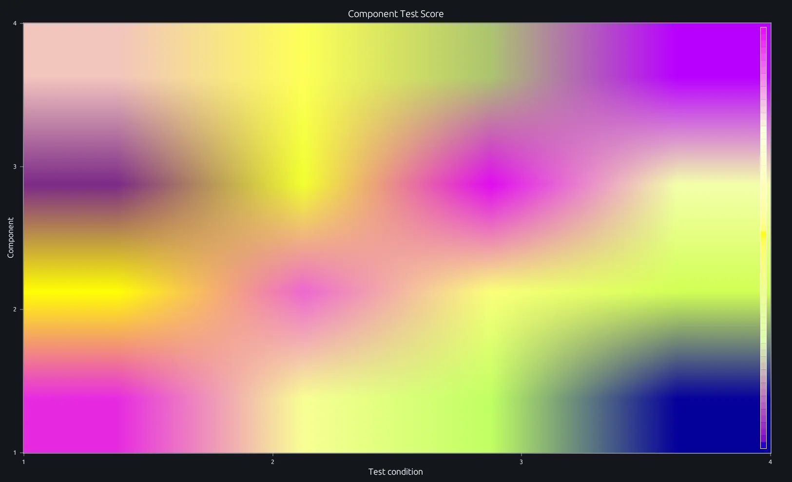
Component test-score matrix rendered as a MATLAB heatmap in RunMat

heatmap

Scan a test matrix for the one condition or channel that behaves differently from the rest.

View MATLAB-syntax code
results = [92 88 81 76; 85 91 87 82; 78 84 93 89; 90 86 80 94];
conditions = {'Cold', 'Nominal', 'Hot', 'Vibration'};
components = {'Pump A', 'Pump B', 'Valve A', 'Valve B'};

h = heatmap(conditions, components, results);
h.Title = 'Component Test Score';
h.XLabel = 'Test condition';
h.YLabel = 'Component';
h.Colormap = 'turbo';
h.ColorbarVisible = true;
View heatmap builtin reference
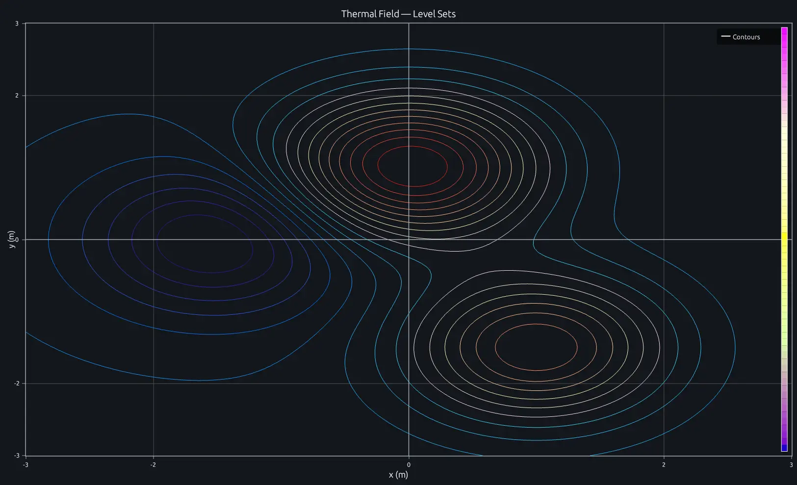
Synthetic thermal field rendered as MATLAB contour lines in RunMat

contour

Follow equal-temperature boundaries across a thermal field without the distortion of perspective.

View MATLAB-syntax code
[X, Y] = meshgrid(linspace(-3, 3, 120), linspace(-3, 3, 120));
Z = 2*exp(-((X-1).^2 + Y.^2)) + 1.5*exp(-((X+1.5).^2 + (Y-1).^2)) - exp(-(X.^2 + (Y+1.5).^2));

contour(X, Y, Z, 20);
colormap('turbo');
colorbar;
title('Thermal Field - Level Sets');
xlabel('x (m)');
ylabel('y (m)');
axis equal;
View contour builtin reference
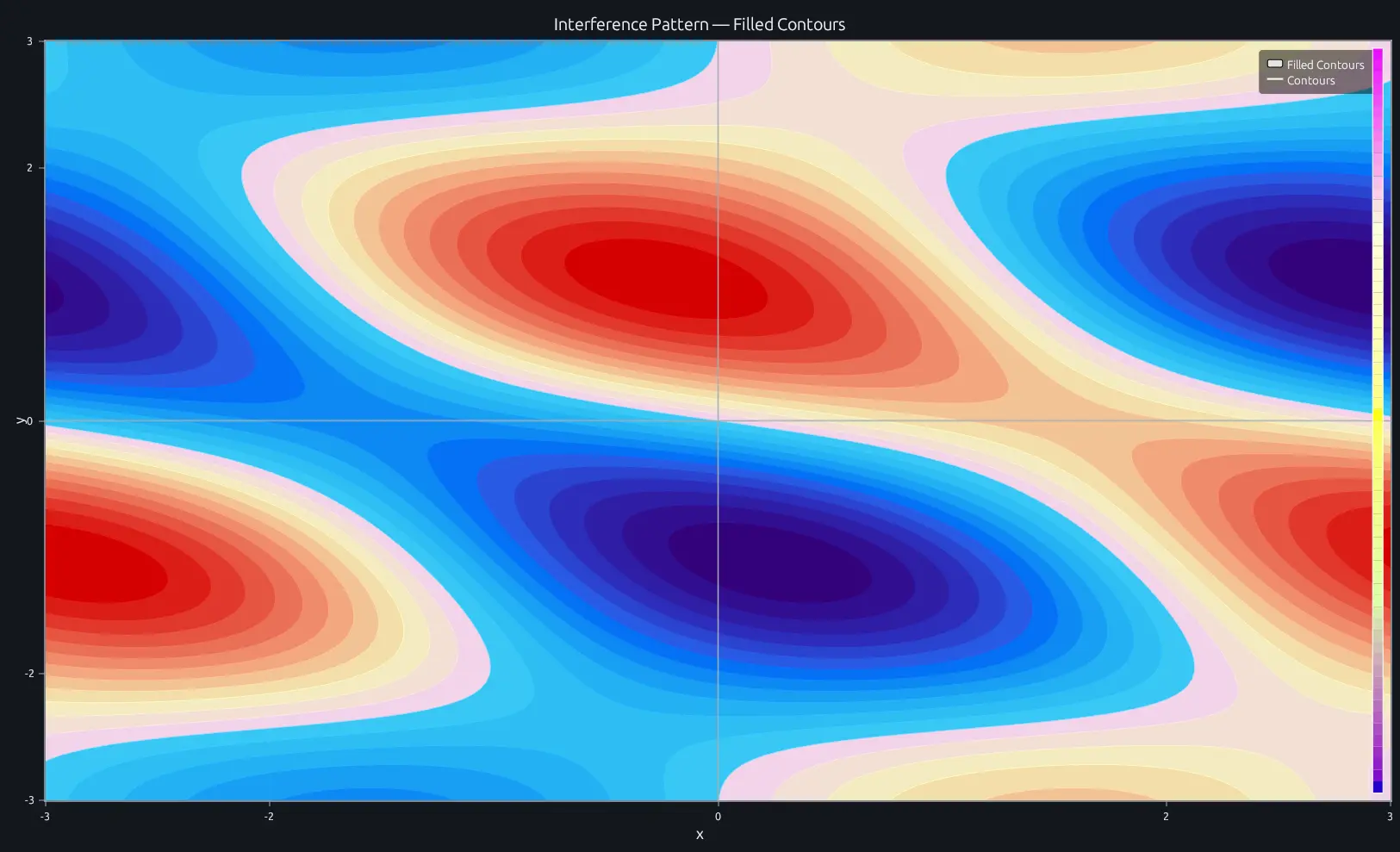
Synthetic interference field rendered as filled MATLAB contours in RunMat

contourf

Separate regions of an interference field into readable value bands.

View MATLAB-syntax code
[X, Y] = meshgrid(linspace(-3, 3, 150), linspace(-3, 3, 150));
Z = sin(X) .* cos(Y) + 0.5*sin(2*X + Y);

contourf(X, Y, Z, 25);
colormap('turbo');
colorbar;
title('Interference Pattern - Filled Contours');
xlabel('x');
ylabel('y');
axis equal;
View contourf builtin reference
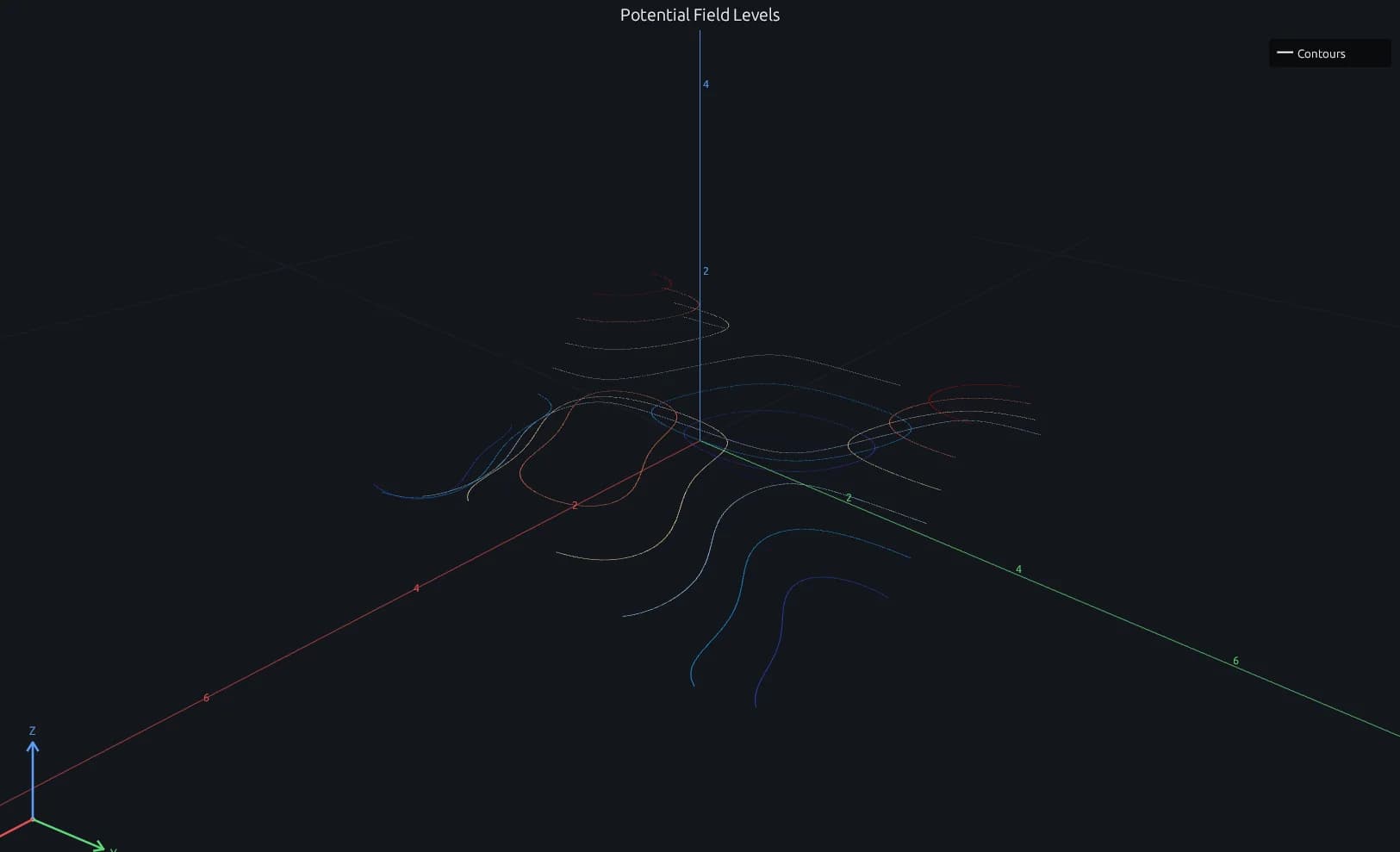
Potential field rendered as elevated MATLAB contour3 level curves in RunMat

contour3

Lift equal-potential lines to their measured levels so their height remains part of the result.

View MATLAB-syntax code
[X, Y] = meshgrid(linspace(-3, 3, 100), linspace(-3, 3, 100));
Z = sin(X).*cos(Y) + 0.25*cos(2*X + Y);
levels = [-0.9 -0.6 -0.3 0 0.3 0.6 0.9];

contour3(X, Y, Z, levels, 'LineWidth', 2);
title('Potential Field Levels');
xlabel('x');
ylabel('y');
zlabel('Potential');
view(42, 28);
grid on;
View contour3 builtin reference
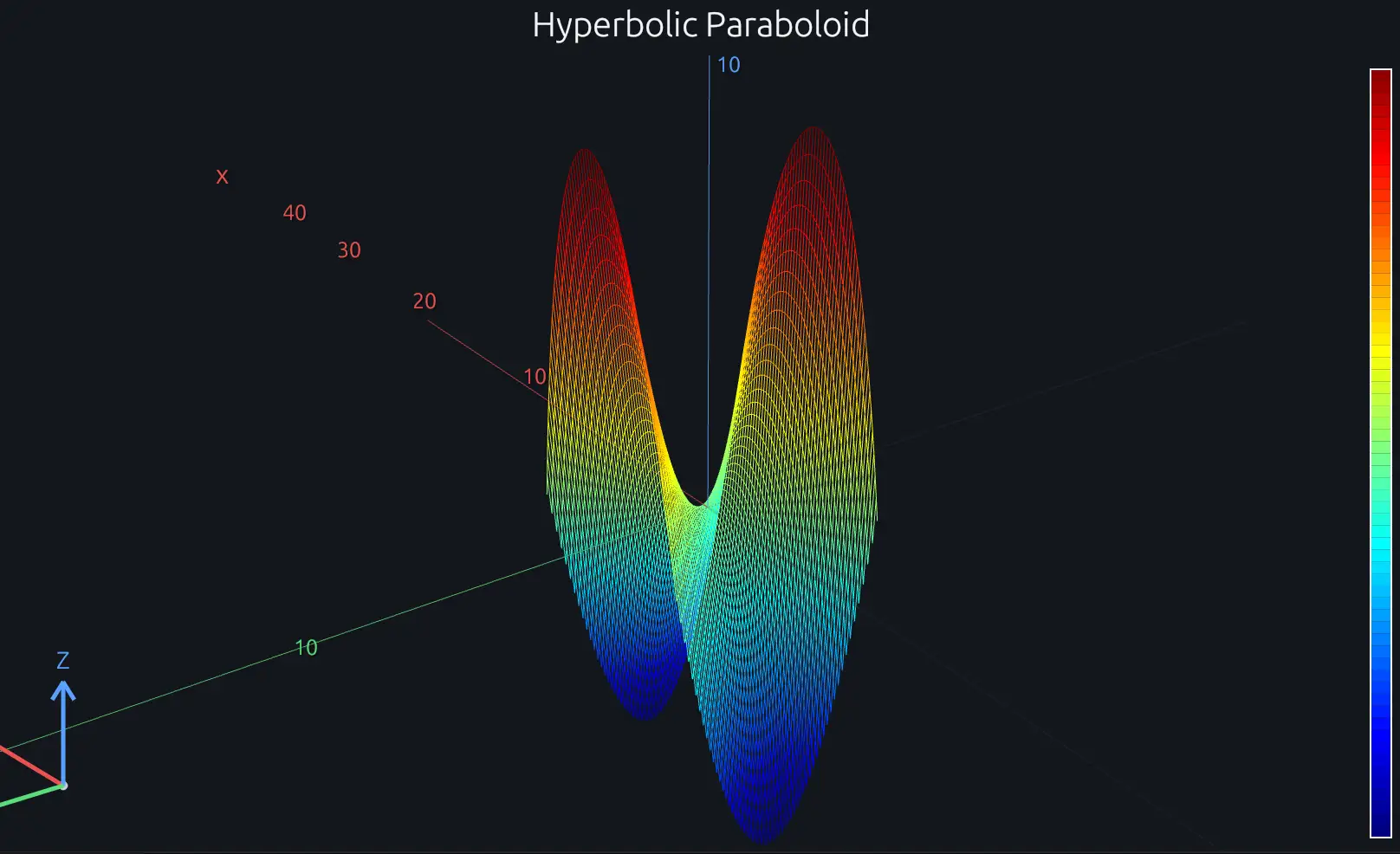
Hyperbolic paraboloid rendered as a MATLAB wireframe mesh in RunMat

mesh

Expose both the saddle shape and the sampling grid behind a response surface.

View MATLAB-syntax code
[X, Y] = meshgrid(linspace(-3, 3, 60), linspace(-3, 3, 60));
Z = X.^2 - Y.^2;

mesh(X, Y, Z);
colormap('jet');
colorbar;
title('Hyperbolic Paraboloid');
xlabel('x');
ylabel('y');
zlabel('z = x^2 - y^2');
view(40, 30);
View mesh builtin reference
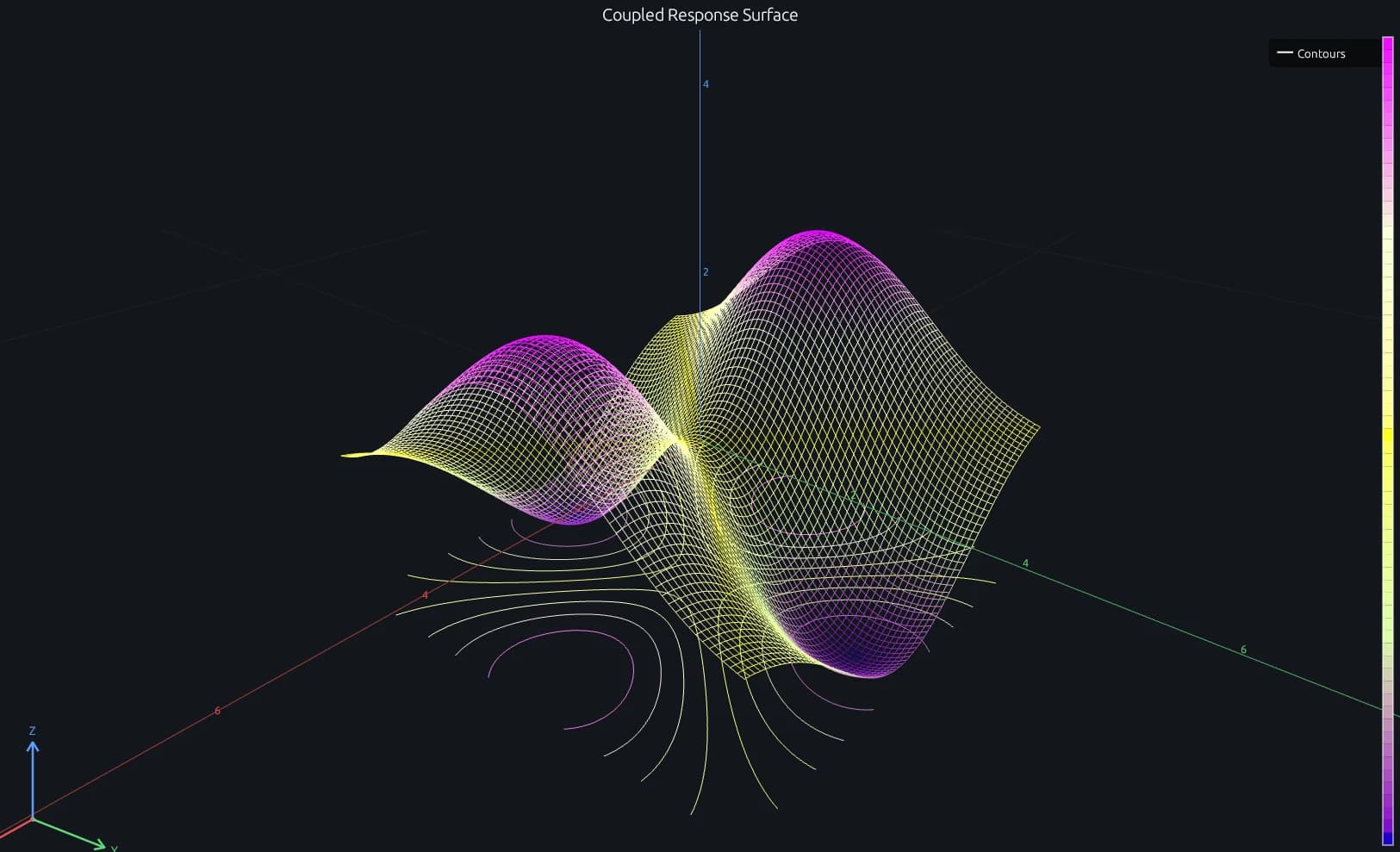
Coupled response surface rendered as a MATLAB mesh with projected contours in RunMat

meshc

Read a response surface in 3-D while keeping its operating regions visible in the contour projection below.

View MATLAB-syntax code
[X, Y] = meshgrid(linspace(-3, 3, 80), linspace(-3, 3, 80));
Z = (X.^2 - Y.^2).*exp(-0.18*(X.^2 + Y.^2));

meshc(X, Y, Z);
colormap('turbo');
colorbar;
title('Coupled Response Surface');
xlabel('x');
ylabel('y');
zlabel('Response');
view(40, 28);
View meshc builtin reference
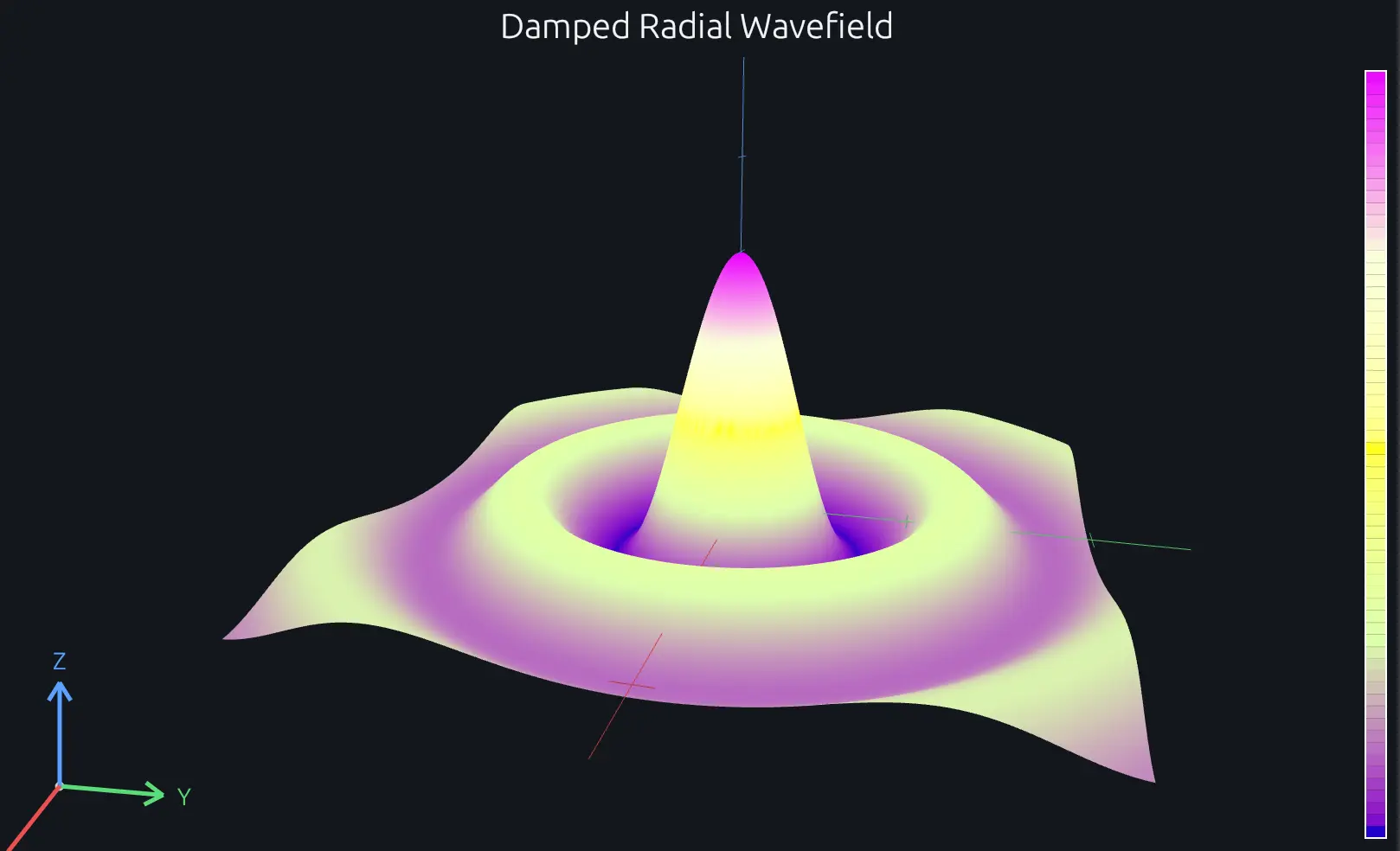
Damped radial wavefield rendered as a shaded MATLAB surface in RunMat

surf

Inspect the peaks, decay, and curvature of a radial wavefield as one continuous surface.

View MATLAB-syntax code
[X, Y] = meshgrid(linspace(-4, 4, 200), linspace(-4, 4, 200));
R = sqrt(X.^2 + Y.^2) + 0.01;
Z = sin(3*R) ./ R;

surf(X, Y, Z);
shading interp;
colormap('turbo');
colorbar;
title('Damped Radial Wavefield');
xlabel('x');
ylabel('y');
zlabel('Amplitude');
view(35, 25);
View surf builtin reference
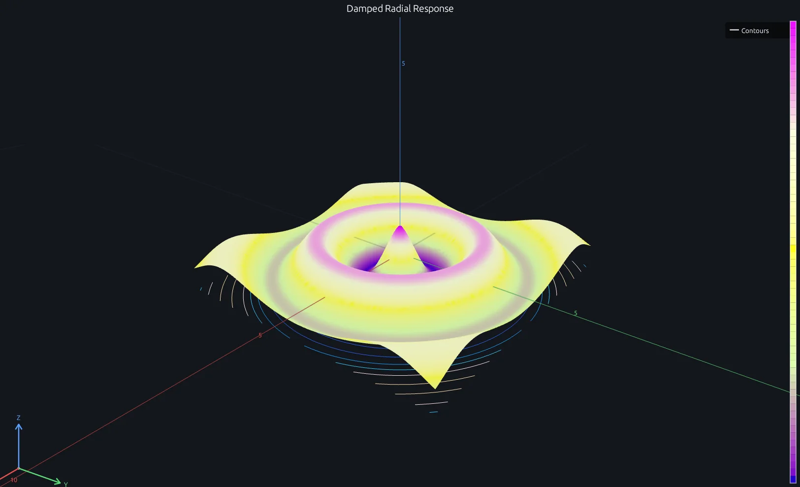
Damped radial response rendered as a MATLAB surface with projected contours in RunMat

surfc

Pair a continuous surface with projected contours when both shape and operating region matter.

View MATLAB-syntax code
[X, Y] = meshgrid(linspace(-4, 4, 120), linspace(-4, 4, 120));
R = sqrt(X.^2 + Y.^2) + 0.15;
Z = cos(2.5*R).*exp(-0.22*R);

surfc(X, Y, Z);
shading interp;
colormap('turbo');
colorbar;
title('Damped Radial Response');
xlabel('x');
ylabel('y');
zlabel('Amplitude');
view(38, 27);
View surfc builtin reference
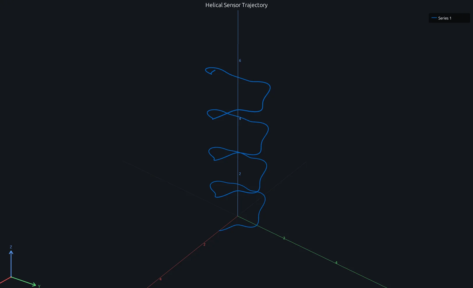
Helical sensor trajectory rendered as a connected MATLAB plot3 path in RunMat

plot3

Follow the ordered path of a sensor as it moves through three-dimensional space.

View MATLAB-syntax code
t = linspace(0, 8*pi, 600);
radius = 1 + 0.12*cos(5*t);
x = radius.*cos(t);
y = radius.*sin(t);
z = linspace(0, 6, 600) + 0.12*sin(3*t);

h = plot3(x, y, z);
set(h, 'LineWidth', 2);
title('Helical Sensor Trajectory');
xlabel('x (m)');
ylabel('y (m)');
zlabel('z (m)');
view(38, 26);
grid on;
axis equal;
View plot3 builtin reference
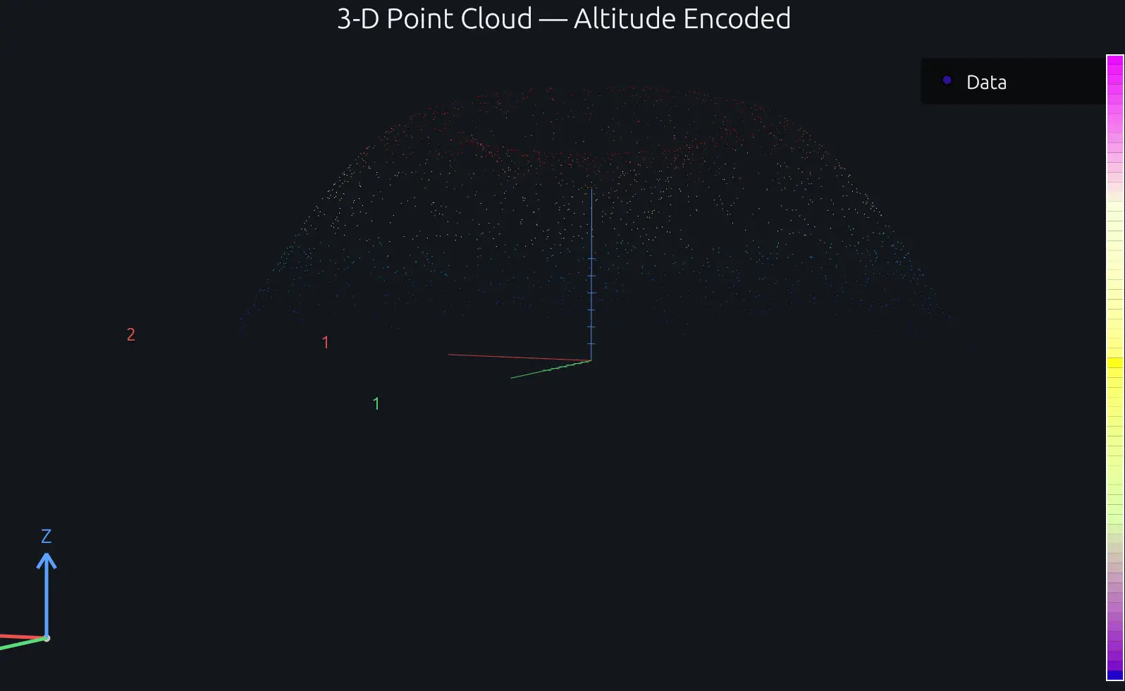
Three-dimensional point cloud colored by altitude and rendered with MATLAB scatter3 in RunMat

scatter3

Inspect a 3-D point cloud while using color to carry a fourth measurement such as altitude.

View MATLAB-syntax code
rng(11);
n = 2000;
theta = 4*pi*rand(1, n);
r = sqrt(rand(1, n));
x = r .* cos(theta);
y = r .* sin(theta);
z = sin(3*r) ./ (1 + r);

scatter3(x, y, z, 12, z, 'filled');
colormap('turbo');
colorbar;
title('3-D Point Cloud - Altitude Encoded');
xlabel('x');
ylabel('y');
zlabel('z');
view(35, 25);
grid on;
View scatter3 builtin reference
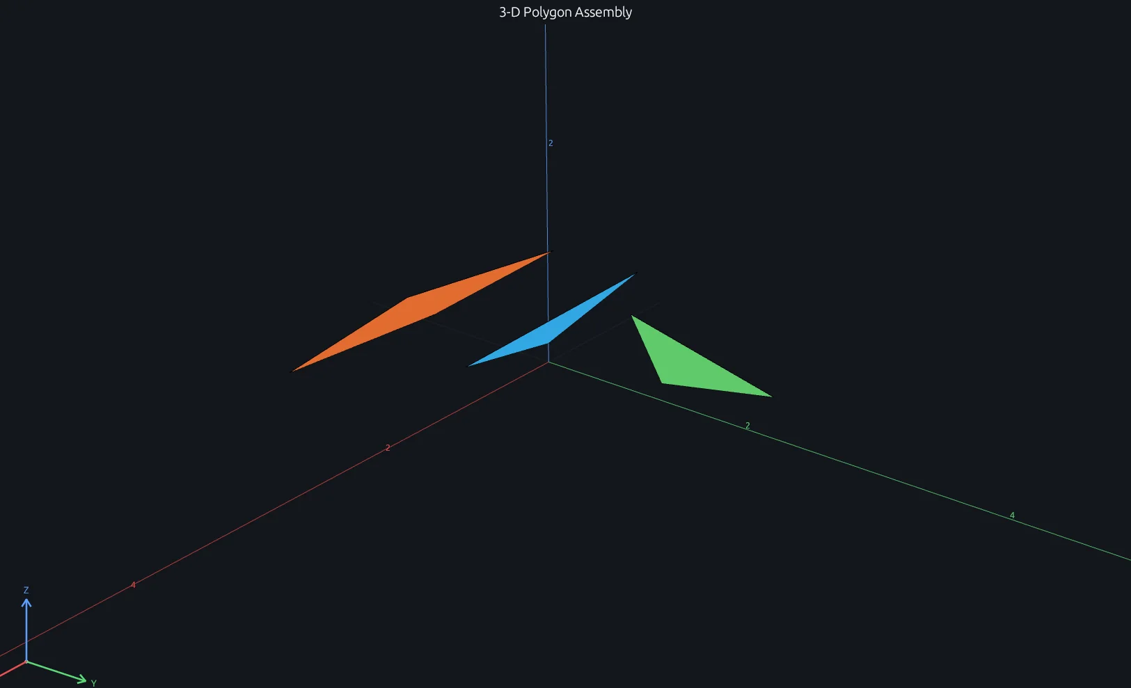
Three separated colored polygons rendered with MATLAB fill3 in RunMat

fill3

Assemble flat colored faces from known vertices to explain a simple 3-D geometry.

View MATLAB-syntax code
x1 = [0 1.3 0.2];
y1 = [0 0.2 1.1];
z1 = [0.2 0.5 1.2];
x2 = [1.5 2.8 2.6 1.4];
y2 = [0.1 0.1 1.1 1.2];
z2 = [1.0 1.0 1.7 1.7];
x3 = [0.4 1.2 0.8];
y3 = [1.5 1.7 2.6];
z3 = [0.4 1.3 0.8];

fill3(x1, y1, z1, [0.2 0.7 0.95], x2, y2, z2, [0.95 0.45 0.2], x3, y3, z3, [0.4 0.85 0.45]);
title('3-D Polygon Assembly');
xlabel('x');
ylabel('y');
zlabel('z');
view(38, 25);
grid on;
View fill3 builtin reference
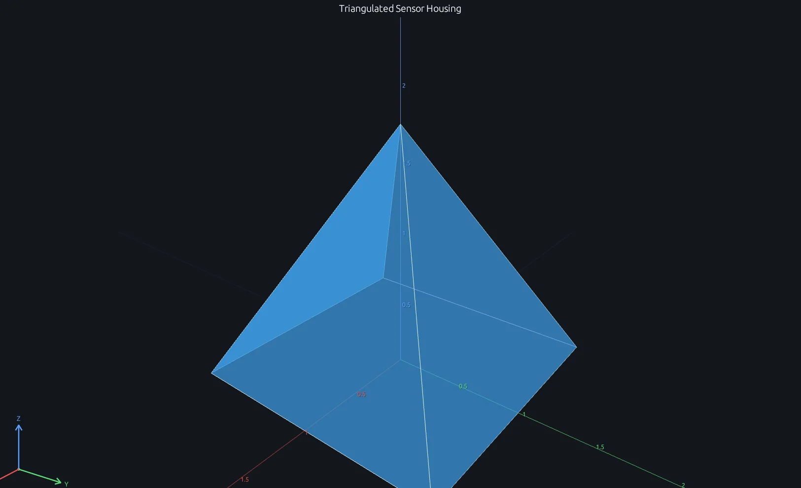
Translucent pyramid geometry rendered from MATLAB patch faces and vertices in RunMat

patch

Build a triangulated housing when the faces, vertices, and appearance need to be controlled directly.

View MATLAB-syntax code
vertices = [-1 -1 0; 1 -1 0; 1 1 0; -1 1 0; 0 0 1.8];
faces = [1 2 5; 2 3 5; 3 4 5; 4 1 5];

patch('Faces', faces, 'Vertices', vertices, 'FaceColor', [0.25 0.65 0.95], 'EdgeColor', [0.9 0.95 1.0], 'FaceAlpha', 0.72);
title('Triangulated Sensor Housing');
xlabel('x');
ylabel('y');
zlabel('z');
view(38, 24);
axis equal;
grid on;
View patch builtin reference
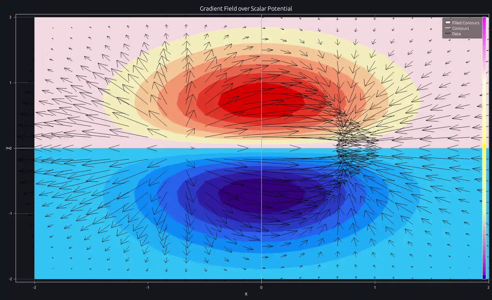
Gradient vectors over a scalar potential rendered with MATLAB quiver and contourf in RunMat

quiver

See which way a gradient points across a scalar field, and how strongly it changes from place to place.

View MATLAB-syntax code
[X, Y] = meshgrid(linspace(-2, 2, 25), linspace(-2, 2, 25));
Z = X .* exp(-X.^2 - Y.^2);
[DX, DY] = gradient(Z, X(1,2)-X(1,1), Y(2,1)-Y(1,1));

contourf(X, Y, Z, 15);
hold on;
quiver(X, Y, DX, DY, 'k', 'LineWidth', 1);
hold off;

colormap('turbo');
colorbar;
title('Gradient Field over Scalar Potential');
xlabel('x');
ylabel('y');
View quiver builtin reference
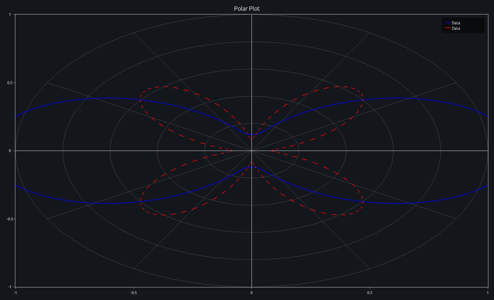
Directional gain response rendered as two MATLAB polarplot series in RunMat

polarplot

Plot antenna gain, directivity, or another response whose natural horizontal coordinate is angle.

View MATLAB-syntax code
theta = linspace(0, 2*pi, 500);
primary = abs(cos(theta)).^3 + 0.12;
secondary = 0.55*abs(sin(2*theta)).^2 + 0.08;

polarplot(theta, primary, 'b-');
hold on;
polarplot(theta, secondary, 'r--', 'LineWidth', 2);
hold off;
View polarplot builtin reference
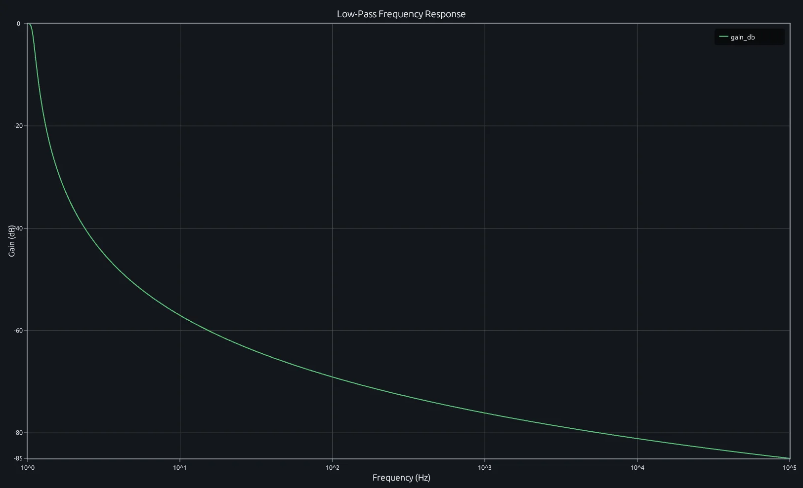
Low-pass frequency response rendered with a logarithmic MATLAB x-axis in RunMat

semilogx

Keep gain readable across a frequency sweep that runs through several orders of magnitude.

View MATLAB-syntax code
frequency = logspace(0, 5, 400);
cutoff = 750;
gain_db = 20*log10(1 ./ sqrt(1 + (frequency/cutoff).^4));

h = semilogx(frequency, gain_db);
set(h, 'LineWidth', 2);
title('Low-Pass Frequency Response');
xlabel('Frequency (Hz)');
ylabel('Gain (dB)');
grid on;
View semilogx builtin reference
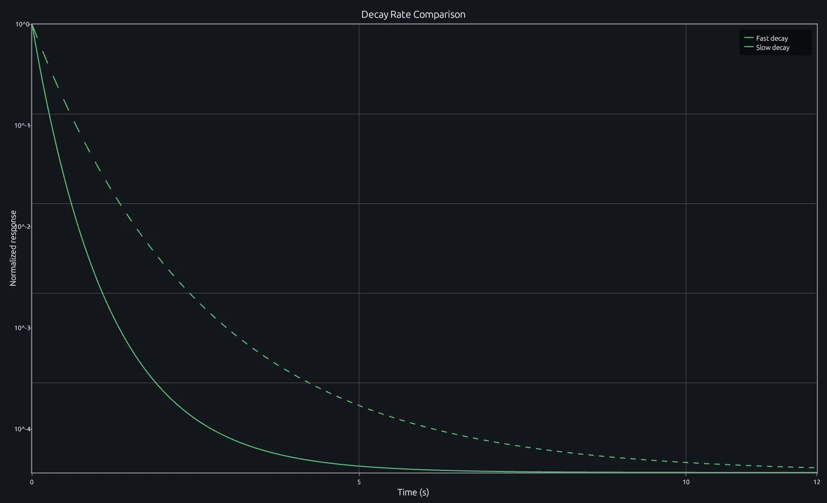
Two exponential decay curves rendered with a logarithmic MATLAB y-axis in RunMat

semilogy

Compare decay rates on a linear time axis even after the responses separate by orders of magnitude.

View MATLAB-syntax code
time = linspace(0, 12, 300);
fast = exp(-0.85*time);
slow = exp(-0.38*time);

h1 = semilogy(time, fast);
set(h1, 'LineWidth', 2, 'DisplayName', 'Fast decay');
hold on;
h2 = semilogy(time, slow, '--');
set(h2, 'LineWidth', 2, 'DisplayName', 'Slow decay');
hold off;
title('Decay Rate Comparison');
xlabel('Time (s)');
ylabel('Normalized response');
legend();
grid on;
View semilogy builtin reference
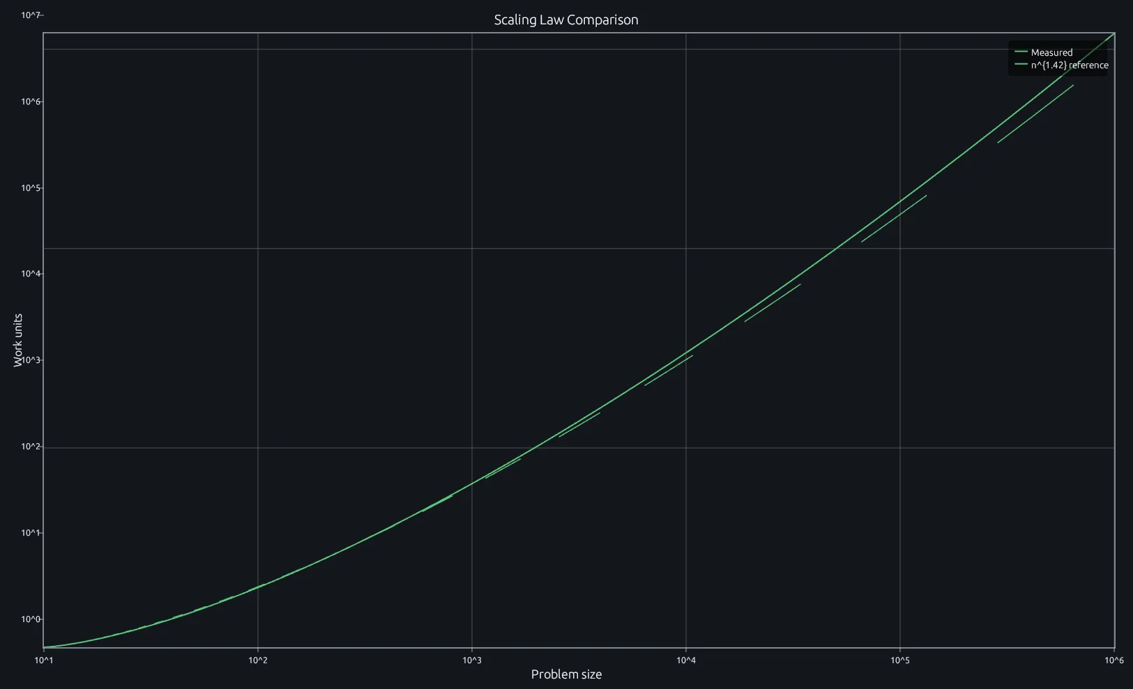
Measured and reference scaling laws rendered with logarithmic MATLAB x and y axes in RunMat

loglog

Check whether two scaling relationships follow a power law across a wide numeric range.

View MATLAB-syntax code
problem_size = logspace(1, 6, 300);
measured = 0.018*problem_size.^1.42 .* (1 + 0.035*sin(log(problem_size)));
reference = 0.018*problem_size.^1.42;

h1 = loglog(problem_size, measured);
set(h1, 'LineWidth', 2, 'DisplayName', 'Measured');
hold on;
h2 = loglog(problem_size, reference, '--');
set(h2, 'LineWidth', 1.5, 'DisplayName', 'n^{1.42} reference');
hold off;
title('Scaling Law Comparison');
xlabel('Problem size');
ylabel('Work units');
legend();
grid on;
View loglog builtin reference
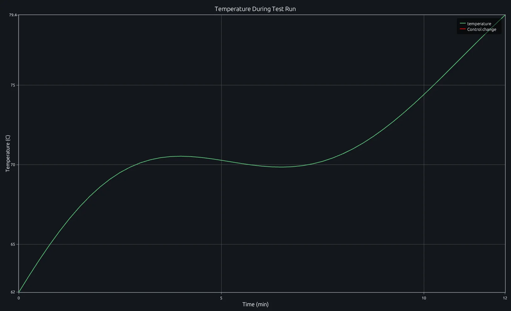
Equipment temperature time series with a vertical MATLAB xline marking a control change in RunMat

xline

Mark the exact moment a test changes state without breaking the measured temperature trace.

View MATLAB-syntax code
time = 0:0.25:12;
temperature = 62 + 1.4*time + 5*sin(0.55*time).*exp(-0.08*time);

plot(time, temperature, 'LineWidth', 2);
xline(6, '--r', 'Control change', 'LineWidth', 1.5);
title('Temperature During Test Run');
xlabel('Time (min)');
ylabel('Temperature (C)');
grid on;
View xline builtin reference
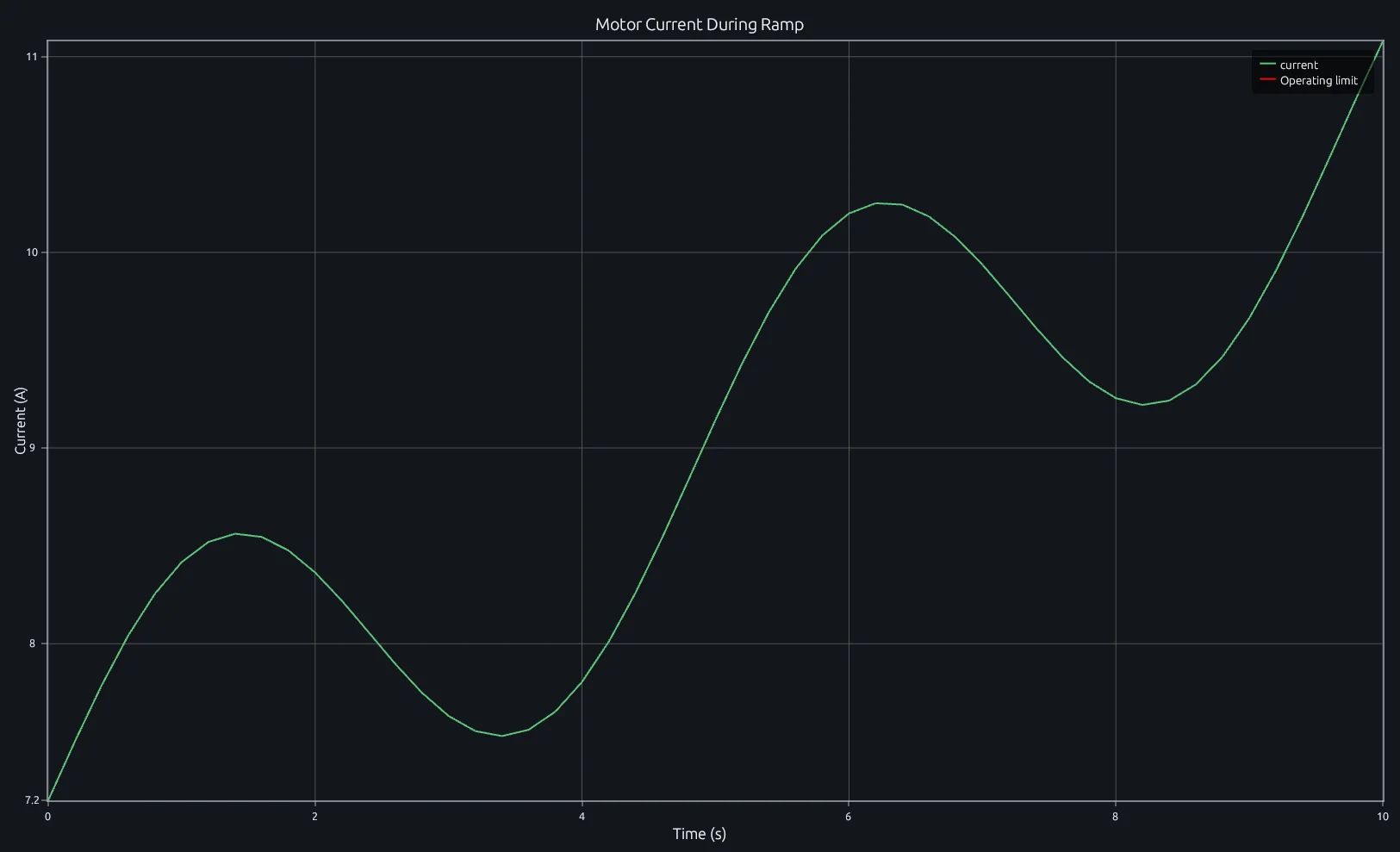
Motor-current time series with a horizontal MATLAB yline marking the operating limit in RunMat

yline

Keep a motor-current limit visible across the full ramp so excursions are obvious.

View MATLAB-syntax code
time = 0:0.2:10;
current = 7.2 + 0.35*time + 0.9*sin(1.3*time);
limit = 11;

plot(time, current, 'LineWidth', 2);
yline(limit, '--r', 'Operating limit', 'LineWidth', 1.5);
title('Motor Current During Ramp');
xlabel('Time (s)');
ylabel('Current (A)');
grid on;
View yline builtin reference

For figure state, styling, and image export, see the MATLAB plotting guide. The builtin reference linked from each card documents the current call forms and supported properties for that function.