
Draw a schematic
This guide draws a barometric pressure sensor board: a 4-pin connector brings in 5 V and an I2C bus, a 3.3 V regulator powers the sensor, pull-up resistors hold the bus lines high, and an LED shows the rail is up. The sensor sits on its own sheet. The result is baro.circuit, which Lay out a board turns into a board.
The Desktop's schematic canvas and the source view edit the same file. Placing a part, drawing a wire or renaming a net on the canvas writes the statements shown here, and typing them redraws the canvas.
1. Place parts
Run New Circuit, or create baro.circuit. Find each part in Search (the left rail) and choose Place; placing writes a component with the part's MPN. A designator ending in ? (R?) is numbered when the schematic is annotated.
sheet main {
    component J1 = { part = "CONN-SH-4P" }
    component U1 = { part = "LDO-3V3-SOT23" }
    component R1 = { part = "R0402-4K7" }
}
A part the built-in library doesn't have is written into the circuit as a part "<mpn>" = { … } declaration, so the file carries every part it uses. See The parts library.
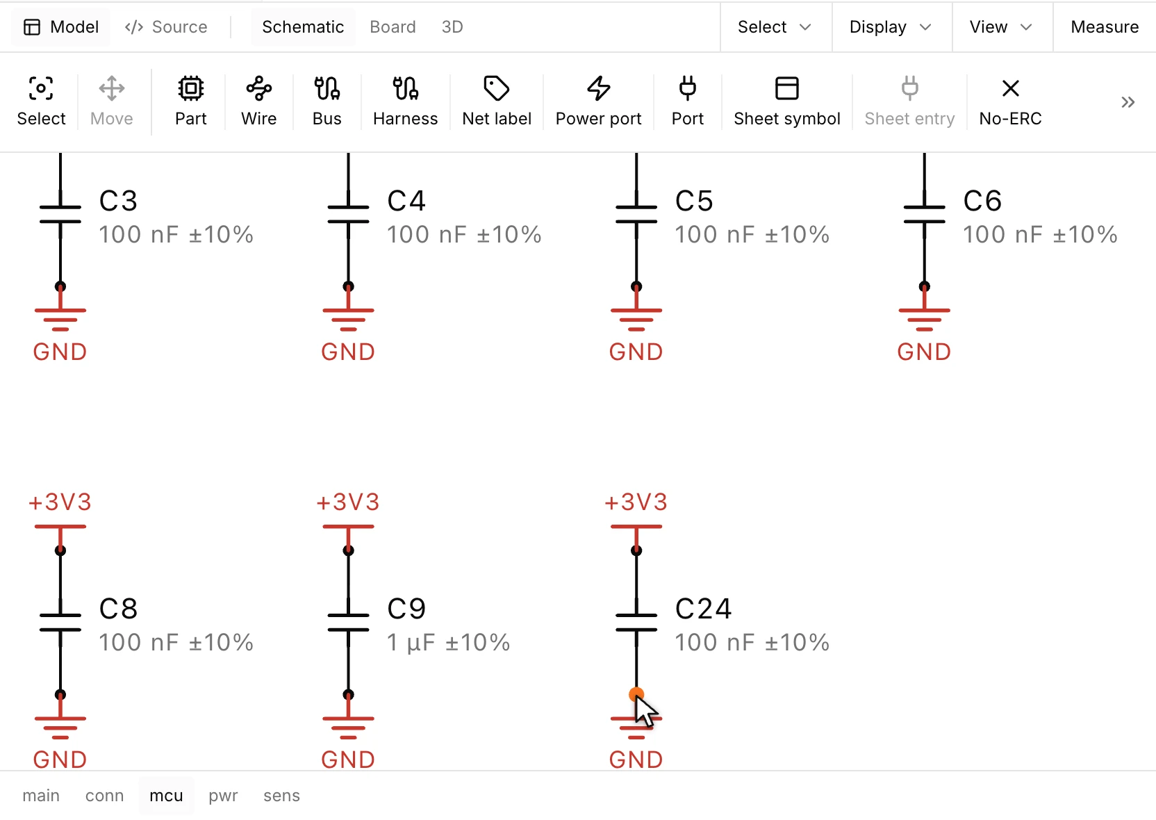
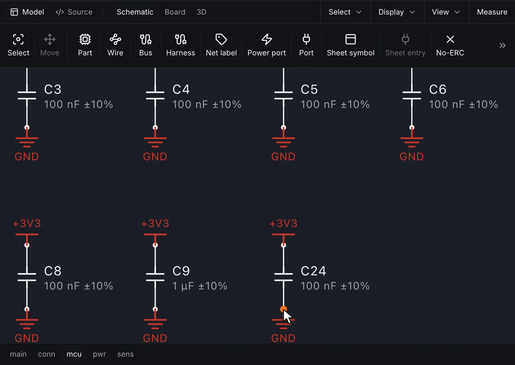
In the Desktop, Part places a component where you click on the sheet, and Power port puts a supply or ground symbol on a pin. Here a 100 nF decoupling capacitor joins the row under the MCU and takes +3V3 and GND:
2. Connect pins into nets
A connect list joins every endpoint it names into one net. A wire drawn on the canvas between two pins adds them to a list. Pins are U1.VIN by name or "J1.1" by number; net.SDA names the net, which needs no declaration unless it has settings.
The canvas routes each wire for you. To route one by hand, click its corners on the empty sheet between the two pins; the Angle setting draws the segments at 90°, at 45° or at any angle, and Shift+Space steps through the three while you draw. The corners are kept in the circuit's lock file, beside the places of the symbols, so the .circuit file still lists only the connection. Moving a part keeps the corners and turns the wire's end once to reach the pin. Removing the connection removes its corners.
A text statement puts a note on the sheet, such as text note1 = "5 V in from J1". The Text tool writes one where you click.
Copying a group of parts and pasting it keeps the wiring inside the group. A net that joins two or more of the copied pins becomes a new net joining their copies, and a copied pin on a rail such as GND joins the same rail. A net that leaves the group stays with the originals, so the copy's pin is left open for you to wire. The Power port tool lists the project's rails as you type its Rail field, and a name that isn't on the list declares a new rail.
Settings go on a net statement:
global = truejoins nets of the same name on every sheet, as ground and supply rails do.power_flag = truemarks a net driven from outside the schematic, such as the 5 V on the connector, so the electrical rules don't report its power inputs as undriven.class = powerputs the net in a net class, whose track width and clearance the board uses.- Other entries are the net's parameters, such as
max_length = 50 mm. The Directive tool's Parameter set writes them onto the picked nets, in the units you type.
To give several nets the same class and parameters, pick them with the Directive tool's Blanket and write a class (power) or entries (class = power, max_length = 50 mm). The tool writes blanket blanket1 = { nets = [VIN, GND], class = power, max_length = 50 mm } on the sheet, and the canvas draws a dashed box round the nets it covers.
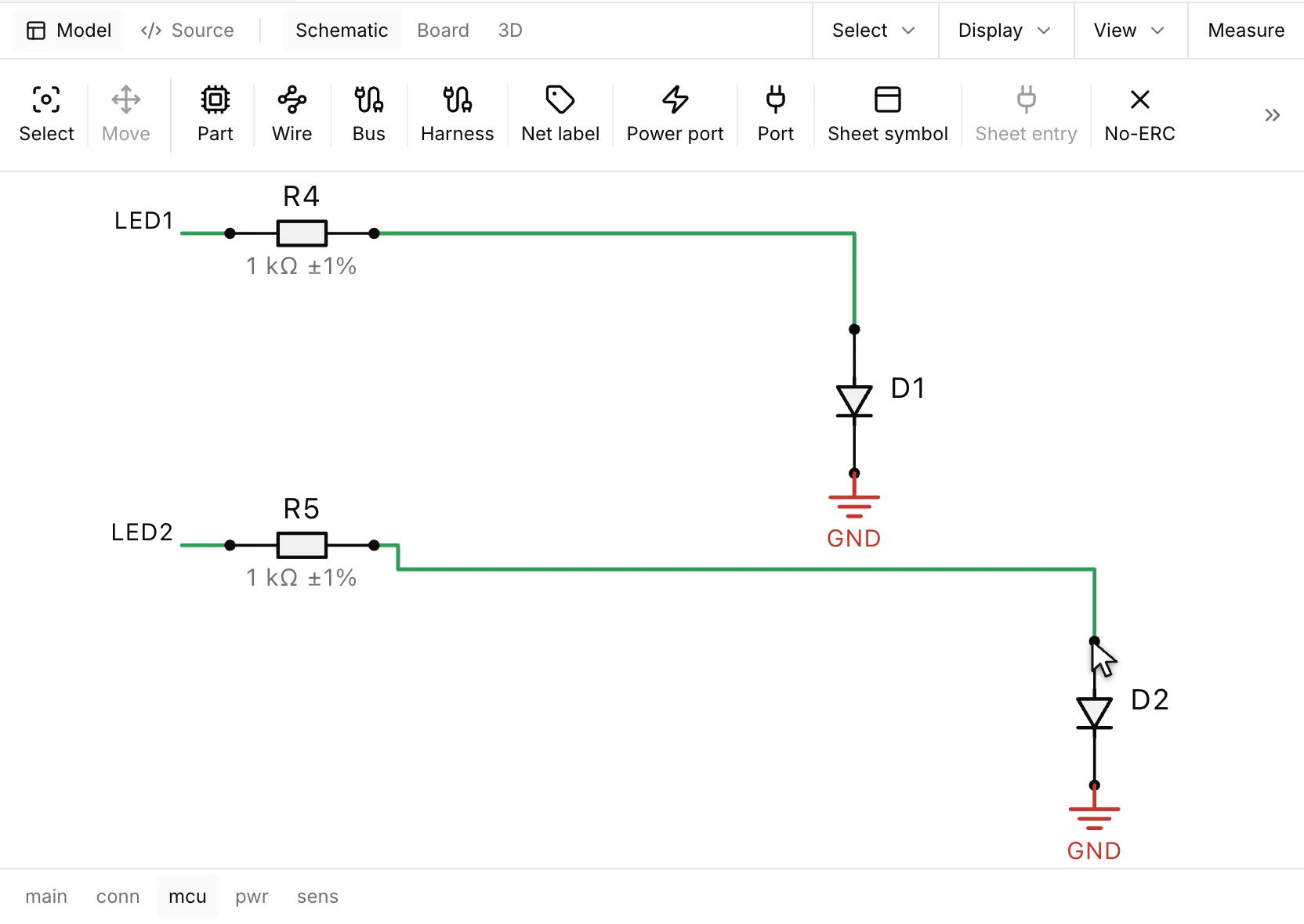
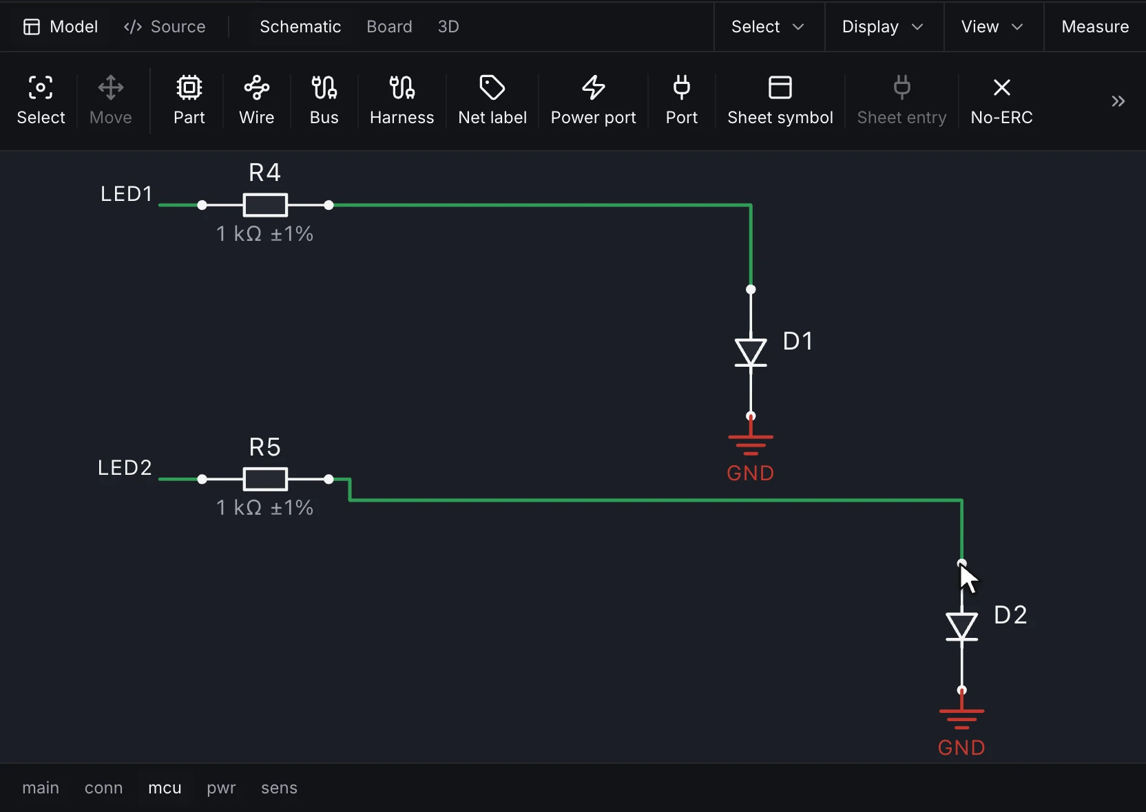
In the Desktop, Wire runs from the pin you click to the next pin you click, across and then up or down, and joins both to one net. Here the second status LED's resistor is wired to the LED's anode, and both unconnected-pin markers clear:
3. Split the design into sheets
A sheet with port statements can be placed in another sheet as a block. Here the sensor and its decoupling capacitor sit on sheet pressure, and sheet main places it once as instance sensor. Endpoints such as instance.sensor.SDA connect the block's ports. On the canvas, the Sheet entry tool adds a port and can bind it in the same step: pick a pin or wire for Bind to and the instance gets bind = { SDA = U1.SDA }. For a repeated sheet, Bus and Offset bind channel i to member offset + i of a bus (bind = { DATA = { bus = D, offset = 0 } }). The +3V3 and GND nets are global, so they reach the sensor sheet with no port. R3's value calls ledResistor.m, which sits beside the circuit (step 4):
function r = ledResistor(vs, vf, i)
% Series resistor that sets an LED's current from its supply and forward voltage (SI).
r = (vs - vf) / i;
end
runmat 0.7
std 1
// A barometric pressure sensor on I2C, powered from a 5 V connector through a 3.3 V regulator.
circuit baro {
root = main
net_class power = { track_width = "0.40 mm", clearance = "0.20 mm" }
sheet main {
component J1 = { part = "CONN-SH-4P" }
component U1 = { part = "LDO-3V3-SOT23" }
component C1 = { part = "C0805-1U" }
component C2 = { part = "C0402-1U" }
component R1 = { part = "R0402-4K7" }
component R2 = { part = "R0402-4K7" }
component R3 = { part = "R0402-1K", value = ledResistor(vs = 3.3 V, vf = 2 V, i = 2 mA) as ohm }
component D1 = { part = "LED0603-G" }
net GND = { class = power, global = true, power_flag = true }
net VIN = { class = power, power_flag = true }
net "+3V3" = { class = power, global = true }
connect = [net.VIN, "J1.1", U1.VIN, U1.EN, "C1.1"]
connect = [net.SDA, "J1.2", "R1.2", instance.sensor.SDA]
connect = [net.SCL, "J1.3", "R2.2", instance.sensor.SCL]
connect = [net.GND, "J1.4", U1.GND, "C1.2", "C2.2", D1.K]
connect = ["net.+3V3", U1.VOUT, "C2.1", "R1.1", "R2.1", "R3.1"]
connect = [net.LED, "R3.2", D1.A]
no_erc = [U1.NC]
instance sensor = { sheet = pressure }
}
sheet pressure {
port SDA : inout
port SCL : in
component U2 = { part = "BARO-LGA8" }
component C3 = { part = "C0402-1U" }
connect = [port.SDA, U2.SDA]
connect = [port.SCL, U2.SCL]
connect = ["net.+3V3", U2.VDD, U2.VDDIO, U2.CSB, "C3.1"]
connect = [net.GND, U2.GND, U2.SDO, "C3.2"]
}
}A sheet can also be placed several times as channels with repeat, each copy with its own designators and nets. See Sheets, hierarchy and channels.
4. Compute a value
R3's value in the circuit above comes from ledResistor.m, the function shown before it, in the circuit's folder. The function sizes the resistor for 2 mA through the LED: .
The arguments arrive in SI units, and as ohm reads the result as a resistance. The circuit keeps the call, so changing the supply or the current recomputes the value. See MATLAB functions in design values.
5. Check it
runmat-design check baro.circuitThe check runs the electrical rules (undriven inputs, conflicting drivers, unconnected pins) and the design-review suites. On this circuit the I2C suite confirms each bus line has a pull-up between 1 kΩ and 10 kΩ, and the decoupling suite confirms each IC power pin has a capacitor to ground. no_erc = [U1.NC] tells the rules the regulator's no-connect pin is meant to be open.
Each finding names its pins and offers a fix where one exists, such as adding the missing capacitor. See Rules and checks.
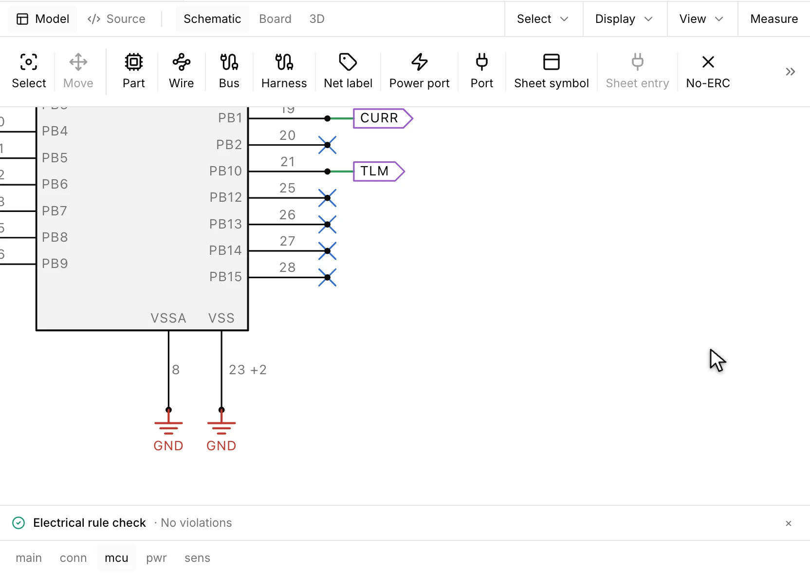
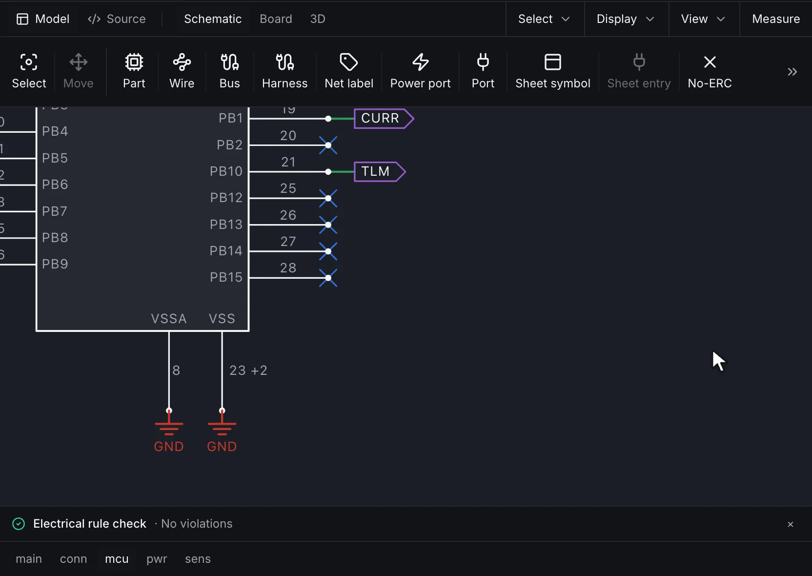
In the Desktop, ERC on the Schematic tab runs the same electrical rules over the whole design and lists each finding under the sheet. Here ERC finds the microcontroller's spare PB15 pin unconnected. PB15 is an unused GPIO, so No-ERC marks it as meant to be open, and the next run ends clean:
6. Move between views
Selecting a component or a net in the schematic selects it on the board and in the 3D board, and the reverse. The board tab follows the schematic: the changes the board hasn't taken are listed until Update board takes them.
Next
- Lay out a board for this circuit.
- Run a circuit simulation adds a simulation section with limits.