
Lay out a board
This guide lays out the pressure sensor from Draw a schematic on a 20 × 15 mm two-layer board. The board lives in baro.circuit.layout beside baro.circuit. The Desktop's board canvas edits it, and every placement, track and via is one line of the file, so a review shows each change line by line.
1. Start the board
Start the board from the circuit's board tab, or create the file. It names its circuit by symbol, then sets the board edge, the layer stack and the fabricator's minimums:
runmat 0.7
std 1

circuit baro {
    root = main
    net_class power = { track_width = "0.40 mm", clearance = "0.20 mm" }

    sheet main {
        component J1 = { part = "CONN-SH-4P" }
        component U1 = { part = "LDO-3V3-SOT23" }
        component C1 = { part = "C0805-1U" }
        component C2 = { part = "C0402-1U" }
        component R1 = { part = "R0402-4K7" }
        component R2 = { part = "R0402-4K7" }
        component R3 = { part = "R0402-1K" }
        component D1 = { part = "LED0603-G" }
        component U2 = { part = "BARO-LGA8" }
        component C3 = { part = "C0402-1U" }
        net GND = { class = power, global = true, power_flag = true }
        net VIN = { class = power, power_flag = true }
        net "+3V3" = { class = power, global = true }
        connect = [net.VIN, "J1.1", U1.VIN, U1.EN, "C1.1"]
        connect = [net.SDA, "J1.2", "R1.2", U2.SDA]
        connect = [net.SCL, "J1.3", "R2.2", U2.SCL]
        connect = [net.GND, "J1.4", U1.GND, "C1.2", "C2.2", D1.K, U2.GND, U2.SDO, "C3.2"]
        connect = ["net.+3V3", U1.VOUT, "C2.1", "R1.1", "R2.1", "R3.1", U2.VDD, U2.VDDIO, U2.CSB, "C3.1"]
        connect = [net.LED, "R3.2", D1.A]
        no_erc = [U1.NC]
    }
}
runmat 0.7
std 1
use circuit baro
layout baro {
outline = [[0, 0], [20, 0], [20, 15], [0, 15]]
limits = { clearance = 0.15, track = 0.15, via_diameter = 0.45, drill = 0.2, annular = 0.1, hole_to_hole = 0.25, copper_to_edge = 0.3, silk_to_pad = 0.1, microvia_drill = 0.1 }
net_class power = { track_width = 0.4 mm, clearance = 0.2 mm }
stackup main {
finish = ENIG
layer "F.Cu" = { kind = copper, thickness = 0.035, weight = 1, material = copper }
layer core = { kind = core, thickness = 1.51, material = fr4 }
layer "B.Cu" = { kind = copper, thickness = 0.035, weight = 1, material = copper }
}
}use circuit barofinds the circuit that a.circuitfile in the same folder declares. A board in another folder addsfrom "./<folder>".outlineis the board edge as a ring of points, in millimeters.limitsholds the fabricator's minimums: clearance, track width, via and drill sizes, annular ring, hole spacing, copper-to-edge and silk-to-pad. Every design-rule finding names the limit it broke and where that limit is written.stackuplists the layers top to bottom. The Layer stack command writes a stackup for a layer count and a board thickness.
To start from a board drawn in another tool, import it; see Import.
2. Take the schematic's components
A new board reports the schematic changes it hasn't taken (board_out_of_sync). Update board takes them in one edit: a footprint for each component, its pads mapped to their nets, and the package of each footprint written into the file so the board is self-contained. The sync section records which footprint is which component:
net GND : power
net "+3V3" : power
footprint C3 = { package = C0402, at = [14.5, 7.5], rotation = 90, pads = { "1" = "+3V3", "2" = GND } }
package C0402 = {
    pads = [
        { number = "1", shape = roundrect, size = [0.5, 0.6], at = [-0.5, 0], layers = smd },
        { number = "2", shape = roundrect, size = [0.5, 0.6], at = [0.5, 0], layers = smd }
    ],
    courtyard = rect([-1, -0.5], [1, 0.5])
}
When the schematic changes later (a part added, a net renamed, a value swapped), the board lists each change, and Update board takes the ones you pick. A component renamed with renamed_from keeps its placement.
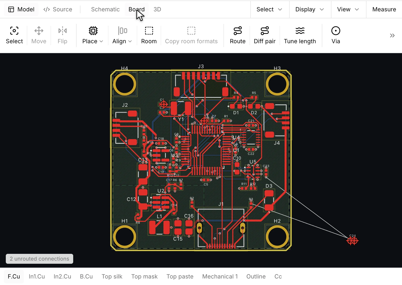
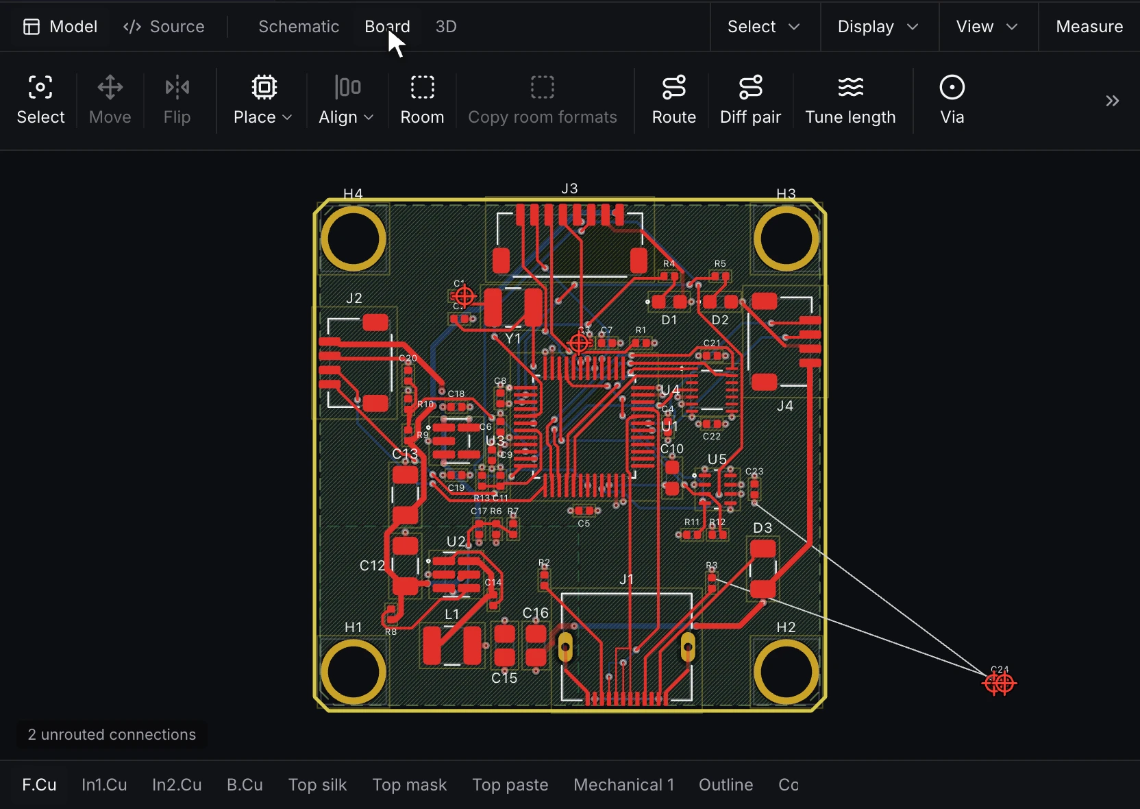
In the Desktop, Update board (ECO) lists each change the board hasn't taken, with its footprint and the sheet it comes from. Apply puts a new component beside the board with its airwires:
3. Place the footprints
Drag footprints on the canvas, or set at, rotation and side in Properties. Place in the order the circuit works: the connector at the board edge, the regulator and its capacitors beside it, the sensor with its decoupling capacitor as close to its supply pins as the courtyards allow, the pull-ups near the connector. Ratsnest lines show the connections still to route. locked = true keeps a placed part from moving.
Placement tools align and distribute a selection, and a room (room <name> = { outline, members }) keeps a group of parts, such as one channel of a repeated sheet, inside an area.
4. Route
Route draws tracks for a net on a copper layer, and a via joins the net's copper on two layers. The width comes from the net's class: power nets take 0.4 mm, the rest take the board's default.
net GND : power
net "+3V3" : power
net SDA
track "+3V3" = { layer = F.Cu, width = 0.4, from = [7, 7.5], to = [11, 7.5] }
track SDA = { layer = F.Cu, width = 0.2, from = [3, 9], to = [11.4, 9] }
via GND = { at = [13, 5], size = 0.6, drill = 0.3 }
pour GND = { name = gnd_bottom, layers = [B.Cu], outline = [[0.5, 0.5], [19.5, 0.5], [19.5, 14.5], [0.5, 14.5]], priority = 1 }- Route net routes one net.
- Diff pair routes a pair declared with
diff_pairin the circuit. Pick either net of the pair. Each net needs one pad at each end. The two tracks leave their pads, merge to the gap you give, and run together at that gap around the board's copper, on the top layer unless you name another. The summary gives each net's length and the skew between them. - Select a net to read its routed length in Properties. A net of a declared pair also shows the other net and the pair's skew. DRC checks each declared pair's gap, its uncoupled length and its skew.
- Tune length adds trombone meanders to a net's longest straight track until the net reaches the target length within the tolerance. Tune the shorter net of a pair to the longer one's length to remove the skew. Meanders only add length, so a net longer than its target needs a shorter route.
- Each of these keeps only copper that passes DRC. When none passes, the command says which finding stopped it and the board is left as it was.
pour GNDfills the bottom layer with ground around everything else; Fill refills pours after an edit.- Vias in the ground pour next to each ground pad (stitching) give the top-layer pads a short path to the plane.
In the Desktop, Route joins the pads you click with a track of the width and layer you give, and Via places a via where you click, on the net of the copper under it. Here C24's two pads are routed to C5's, and a stitching via on the new ground track joins it to the In1.Cu ground plane:
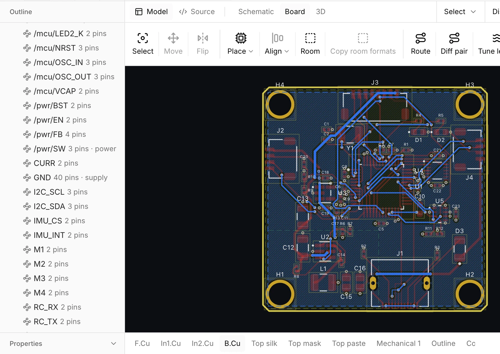
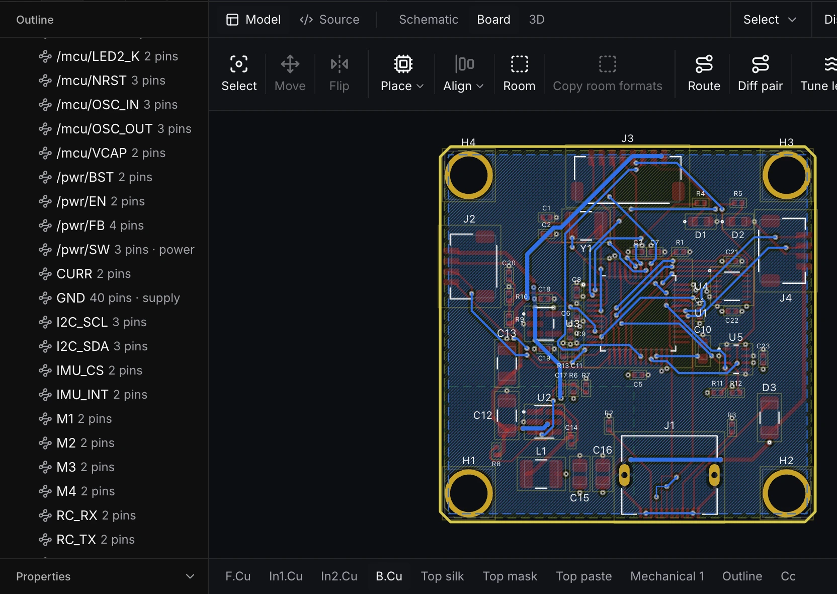
Draw pour takes a net, the corners of its outline and a layer, and fills that layer with the net, clear of every other net's copper. Here GND fills the bottom layer:
5. Clear the design-rule check
DRC runs as you edit. Each finding names the rule, the two objects and the gap between them, and selecting it selects those objects on the canvas. Typical findings are a track too close to a pad of another net, copper too near the edge, silkscreen on a pad, an unrouted connection. The check passes when DRC is clean, every connection is routed and the board has taken every schematic change:
runmat-design check baro.circuit.layoutSee Board layout for every rule.
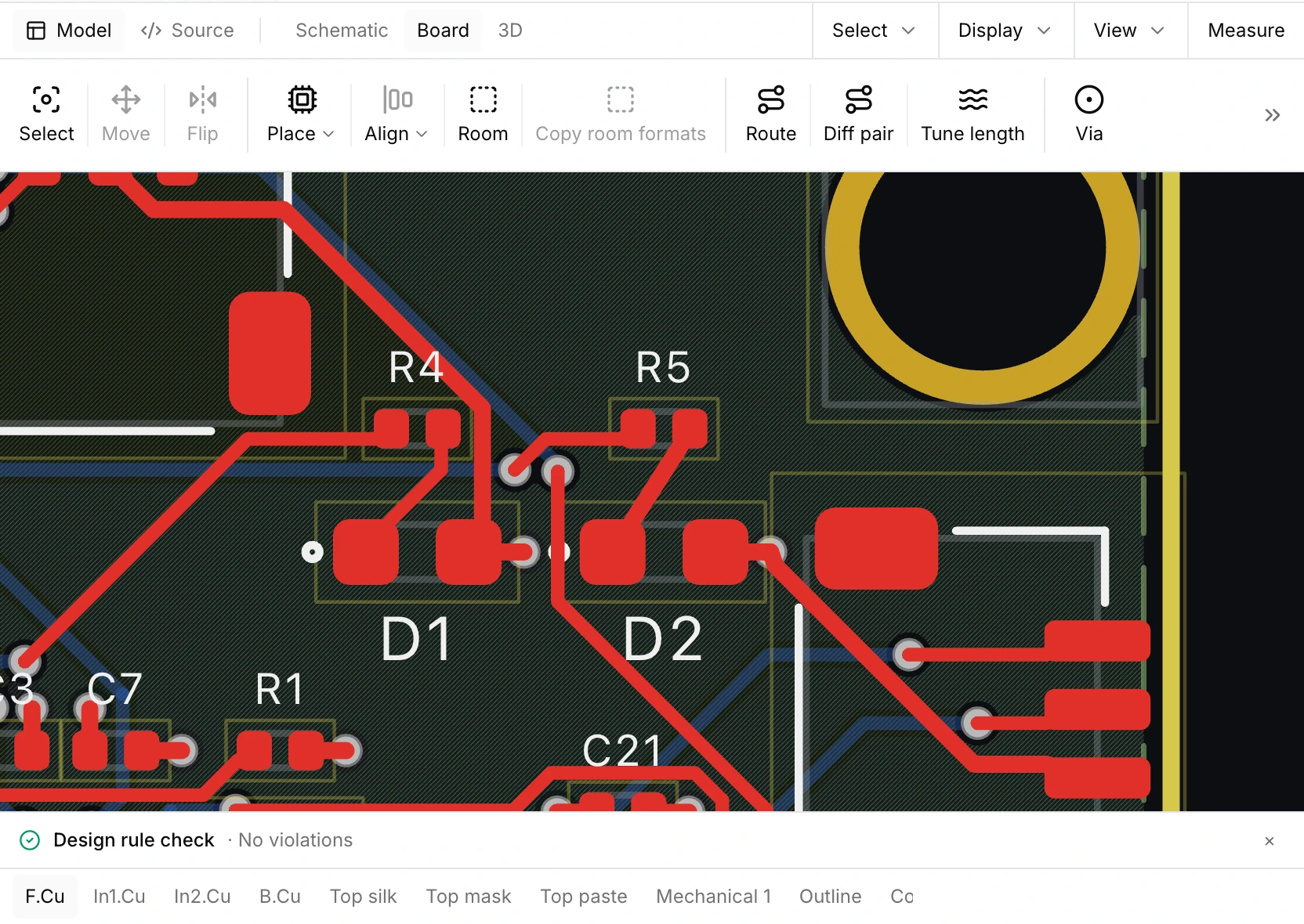
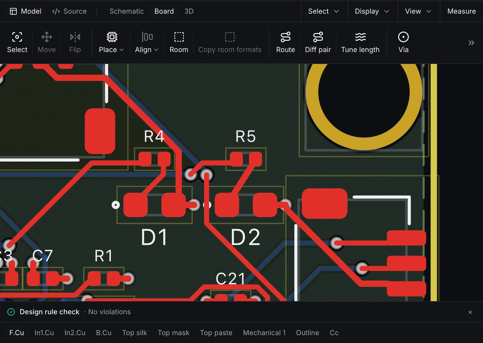
In the Desktop, DRC on the Board tab runs the full check and lists each finding under the board. Here DRC finds the LED2_K net in two pieces, D2's cathode pad and R5. Route joins the two pads, and the next run ends clean:
6. See it in 3D
The 3D board tab shows the stackup, copper and component bodies. An assembly places the board as a part, and selecting a component in 3D selects it on the schematic and the board. A board placed in its enclosure checks the fit of its components against the enclosure's parts Not yet releasedStatus.
Next
- Make fabrication outputs for this board.
- Board layout lists every board statement.