
Finite-element analysis
Linear static analysis
Predict deformation and stress under steady loading. Create a structural study, explore its results, and open the complete example in RunMat Desktop.
A linear static analysis finds the displacement, strain and stress in a supported part under loads that do not change with time. It applies while strains stay small, the material stays elastic and contacts neither open nor close. This page works one example in full: the theory a mechanics-of-materials course teaches, the finite-element method that generalizes it, and the solution in RunMat.
Example 1: A steel cantilever under an end load
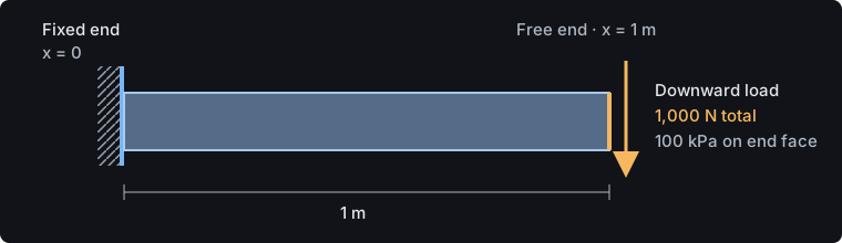
A steel cantilever is built into a rigid wall at one end and loaded downward at the other. The design must keep the tip deflection within L/2,000 and the bending stress below an allowable of 167 MPa (yield strength 250 MPa with a factor of safety of 1.5).
Given
| Quantity | Value |
|---|---|
| Length | L = 1 m, along x from the wall |
| Cross-section | square, b = h = 100 mm |
| Material | steel, E = 200 GPa, ν = 0.3 |
| Support | the face at x = 0 is fixed in all directions |
| Load | P = 1,000 N downward (−z), spread uniformly over the end face at x = L as a traction of 100 kPa |
| Deflection limit | L/2,000 = 0.5 mm |
| Allowable stress | 167 MPa |
Find
- The tip deflection.
- The bending stress near the support.
- The force and moment the wall carries.
- Whether the beam meets the deflection limit and the allowable stress.
Bending of a cantilever beam
Assumptions
Euler–Bernoulli beam theory assumes that plane cross-sections stay plane and normal to the deflected axis, that deflections and rotations are small, and that the material is linear elastic. The first assumption neglects shear deformation, which is reasonable for a slender beam: this one has L/h = 10, and shear adds under 1 % to its deflection.
Governing equations
With the downward deflection, the bending moment and the curvature are related by , and equilibrium of a beam element with no distributed load gives
The wall fixes the deflection and the slope, and the free end carries the shear force P and no moment:
Integrating four times and applying these conditions gives the deflected shape, the tip deflection and the moment:
The bending stress varies linearly through the depth and is largest on the top and bottom surfaces, at a distance from the neutral axis:
For this beam, , so mm, the stress at the wall is 6.0 MPa, and the wall carries a force of 1,000 N and a moment of 1,000 N·m. These are the sizes of answer to expect.
Finite-element formulation
Beam theory needs a slender, prismatic member. The finite-element method solves the equilibrium of the full three-dimensional solid, so the same steps apply to a bracket or a casting where no formula exists.
Field equations. Linear elasticity relates the displacement , the strain and the stress:
with on the fixed face and on the loaded face . For an isotropic material, depends only on and .
Weak form. Multiplying the equilibrium equation by a virtual displacement that vanishes on and integrating by parts gives the principle of virtual work:
Shape functions. The solid is divided into ten-node tetrahedra (Tet10): four corner nodes and six mid-edge nodes. In volume coordinates (with ), the shape functions are quadratic:
and the displacement inside an element is interpolated from its nodal values, . A quadratic displacement gives a strain that varies linearly across the element, which is exactly how bending strain varies through a beam's depth.
Element matrices. Writing the strain in terms of nodal displacements, , turns the weak form into element stiffness matrices and load vectors:
where is the elasticity matrix. Each is 30 × 30 (ten nodes, three displacements each) and is integrated with four Gauss points.
Assembly and supports. Summing the element contributions into global positions gives
The fixed face prescribes on its nodes. Partitioning the unknowns into free (f) and constrained (c) sets,
where are the support reactions. Once the part is supported, is symmetric positive definite, and RunMat solves it with a sparse Cholesky factorization.
Stress recovery. Stress follows from the solved displacements, , at the four Gauss points of each element. The element stress is their volume-weighted average; the nodal stress extrapolates the Gauss-point values to the nodes and averages them between neighboring elements of the same material. The von Mises stress combines the components into one scalar, , where is the deviatoric stress. The structural physics reference covers the other structural procedures.
Solution
The study file states the geometry, mesh, material, support, load and requested results. Each block below is an excerpt of cantilever-static.fea.
Geometry
The beam is imported from a STEP file. Its faces carry names in the CAD, so the study refers to "Fixed end" and "Loaded end" instead of face numbers that change when the CAD is edited.
geometry beam {
    file = "./geometry/cantilever.step"
    units = mm
    region body : solid { select name "Beam"; expect exactly_one }
    region fixed_end : face { select name "Fixed end"; expect exactly_one }
    region loaded_end : face { select name "Loaded end"; expect exactly_one }
}
expect exactly_one makes runmat check stop with a located message if a face is renamed or missing.
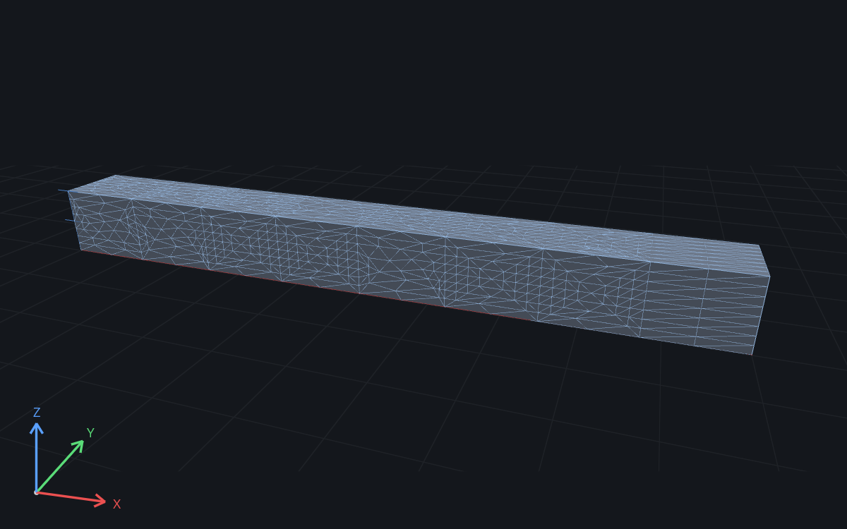
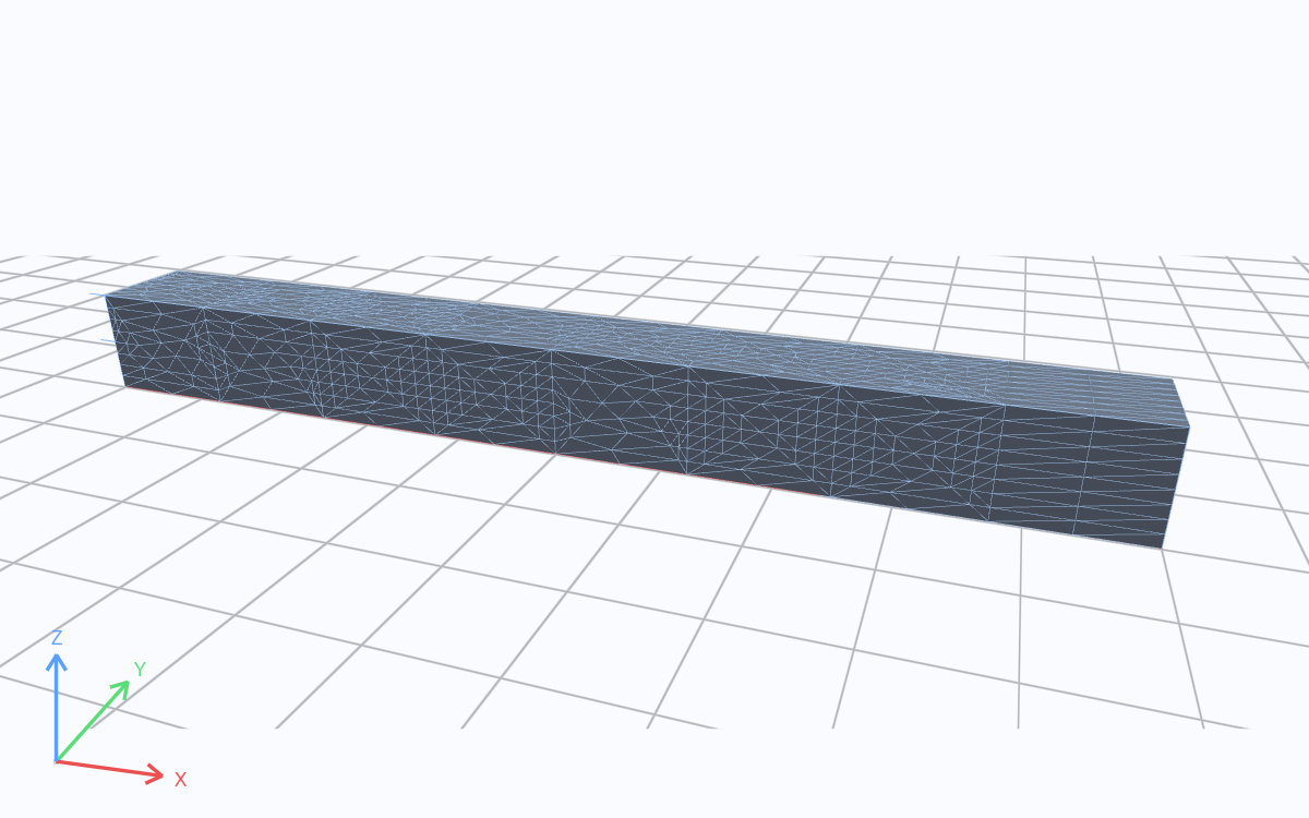
Solver mesh · m. Drag to rotate; scroll to zoom.
Material
A linear static analysis needs only the elastic constants E and ν. The density is unused here; it serves gravity loads and modal studies of the same part.
material steel {
    mass_density = 7850 kg/m^3
    elastic {
        youngs_modulus = 200 GPa
        poisson_ratio = 0.3
    }
}
Support and load
structural.fixed sets every displacement component on the end face to zero: the of the formulation. The 1,000 N load is applied as a traction, 1,000 N over the 0.01 m² end face, or 100 kPa. The traction enters through the face integral above, which spreads it over the face nodes consistently. A force at a single node would instead produce an unbounded stress beneath it.
model loaded_beam {
    assign material.steel to geometry.beam.region.body
    constraint fixed_end {
        structural.fixed { target = geometry.beam.region.fixed_end }
    }
    load end_traction {
        traction on geometry.beam.region.loaded_end = [0, 0, -100000] Pa
    }
    load_case service { include load.end_traction }
}
Mesh
Quadratic tetrahedra are chosen because the part bends: one Tet10 element already represents the linear variation of strain through the depth. A linear tetrahedron (Tet4) has constant strain, cannot bend within one element, and makes a bending part too stiff unless the mesh is very fine. A 150 mm target size gives 1,510 elements and 2,727 nodes, about 8,200 unknowns.
mesh beam on geometry.beam {
    tetrahedra {
        order = quadratic
        target_size = 0.15 m
        maximum_deviation = 0.001 m
    }
}
maximum_deviation limits how far the mesh surface may depart from the CAD surface. It matters on curved parts and has no effect on this flat-sided beam.
Study and outputs
The study selects a static structural analysis and names the results to publish: the displacement field, the element von Mises stress, the tip deflection, and a check of the tip deflection against the 0.5 mm limit.
study cantilever_static {
    geometry = geometry.beam
    mesh = mesh.beam
    model = model.loaded_beam
    analysis static { structural static {} }
    output displacement = analysis.static.field.node.displacement
    output von_mises = analysis.static.field.element.von_mises_stress
    output tip_deflection = max(magnitude(analysis.static.field.node.displacement), over = geometry.beam.region.loaded_end)
    assessment deflection_limit {
        value = output.tip_deflection
        maximum = 0.5 mm
        evidence = authored_samples
    }
}
Run
The complete example opens in RunMat Desktop with its source, the STEP file and saved results:
Import the geometry and choose the mesh
geometry beam {
    file = "./geometry/cantilever.step"
    units = mm
    region body : solid { select name "Beam"; expect exactly_one }
    region fixed_end : face { select name "Fixed end"; expect exactly_one }
    region loaded_end : face { select name "Loaded end"; expect exactly_one }
}

mesh beam on geometry.beam {
    tetrahedra {
        order = quadratic
        target_size = 0.15 m
        maximum_deviation = 0.001 m
    }
}
Choose an elastic material
material steel {
    mass_density = 7850 kg/m^3
    elastic {
        youngs_modulus = 200 GPa
        poisson_ratio = 0.3
    }
}
Fix one end and apply the load
model loaded_beam {
    assign material.steel to geometry.beam.region.body
    constraint fixed_end {
        structural.fixed { target = geometry.beam.region.fixed_end }
    }
    load end_traction {
        traction on geometry.beam.region.loaded_end = [0, 0, -100000] Pa
    }
    load_case service { include load.end_traction }
}
Request the analysis and result fields
study cantilever_static {
    geometry = geometry.beam
    mesh = mesh.beam
    model = model.loaded_beam
    analysis static { structural static {} }
    output displacement = analysis.static.field.node.displacement
    output von_mises = analysis.static.field.element.von_mises_stress
    output tip_deflection = max(magnitude(analysis.static.field.node.displacement), over = geometry.beam.region.loaded_end)
    assessment deflection_limit {
        value = output.tip_deflection
        maximum = 0.5 mm
        evidence = authored_samples
    }
}Includes the study, STEP geometry, and saved results. Run new analyses in RunMat Desktop or the CLI.
View the complete study
// Engineering physics belongs in the importing study.

geometry beam {
    file = "./geometry/cantilever.step"
    units = mm
    region body : solid { select name "Beam"; expect exactly_one }
    region fixed_end : face { select name "Fixed end"; expect exactly_one }
    region loaded_end : face { select name "Loaded end"; expect exactly_one }
}

mesh beam on geometry.beam {
    tetrahedra {
        order = quadratic
        target_size = 0.15 m
        maximum_deviation = 0.001 m
    }
}

material steel {
    mass_density = 7850 kg/m^3
    elastic {
        youngs_modulus = 200 GPa
        poisson_ratio = 0.3
    }
}

model loaded_beam {
    assign material.steel to geometry.beam.region.body
    constraint fixed_end {
        structural.fixed { target = geometry.beam.region.fixed_end }
    }
    load end_traction {
        traction on geometry.beam.region.loaded_end = [0, 0, -100000] Pa
    }
    load_case service { include load.end_traction }
}

study cantilever_static {
    geometry = geometry.beam
    mesh = mesh.beam
    model = model.loaded_beam
    analysis static { structural static {} }
    output displacement = analysis.static.field.node.displacement
    output von_mises = analysis.static.field.element.von_mises_stress
    output tip_deflection = max(magnitude(analysis.static.field.node.displacement), over = geometry.beam.region.loaded_end)
    assessment deflection_limit {
        value = output.tip_deflection
        maximum = 0.5 mm
        evidence = authored_samples
    }
}
From the command line, in the example folder:
runmat check cantilever-static.fea
runmat run cantilever-static.fea
check catches unit mistakes, broken references and missing CAD names in a few seconds, before any meshing. run imports the STEP file, meshes, assembles and solves , recovers stress, and publishes the outputs. See check, plan and run.
Reactions
The reactions at the fixed face sum to 1,000 N upward, equal and opposite to the applied load. Checking this first catches a load on the wrong face, a unit error or a support that restrains too much. Taking moments about the wall, the same reactions carry a moment of P L = 1,000 N·m.
Deflection
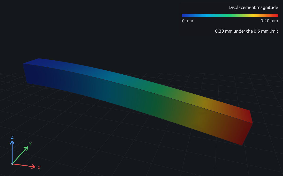
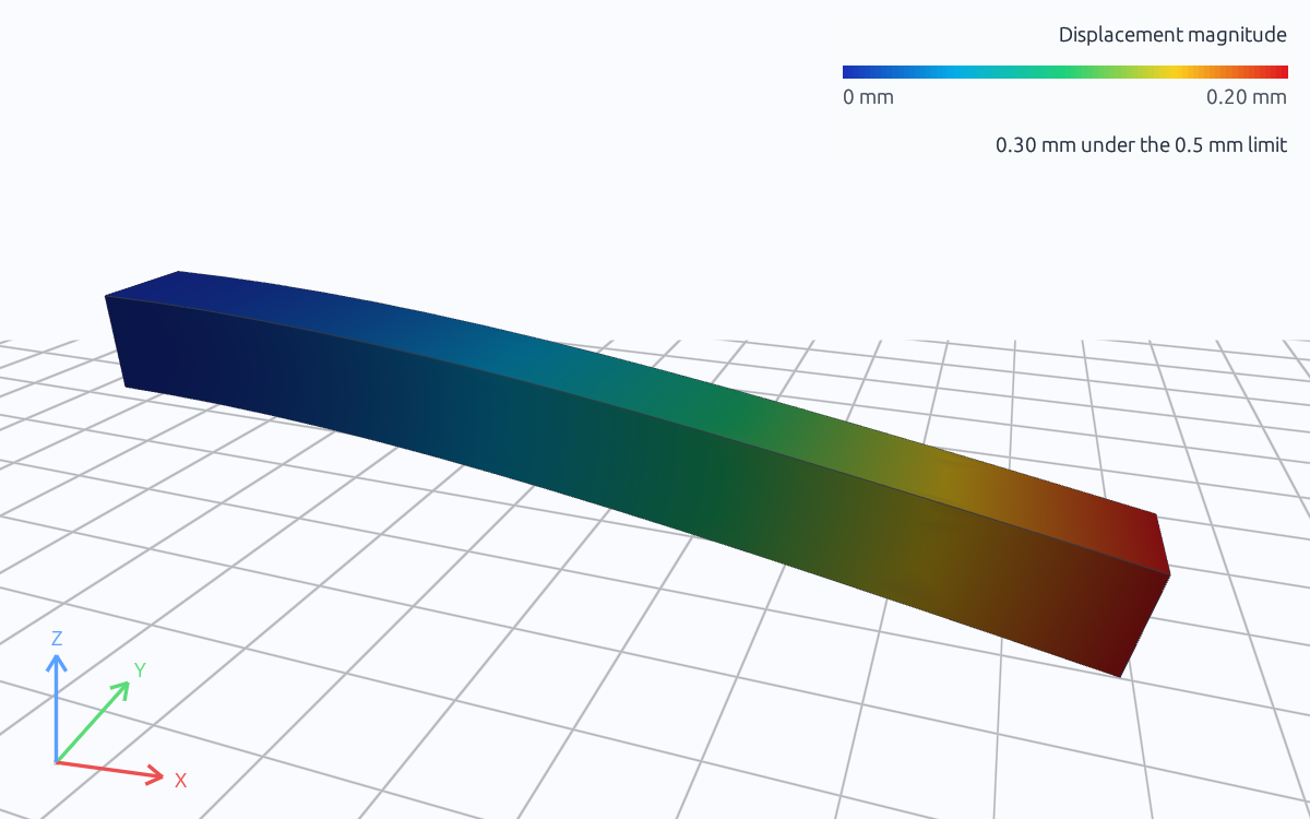
Displacement magnitude · m · 0.00 to 0.000200 · displayed deformation scale 606×. Drag to rotate; scroll to zoom.
Color shows the displacement magnitude, and the shape is exaggerated so the bending is visible. The free end drops and the beam curves smoothly from the wall, the shape above. The tip moves down by 0.2000 mm, the tip_deflection output, and the deflection_limit assessment passes.
Stress
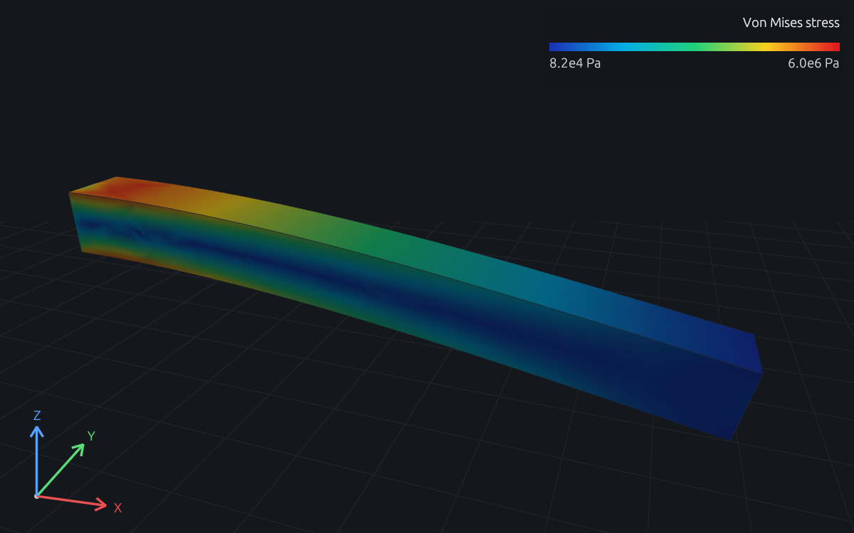
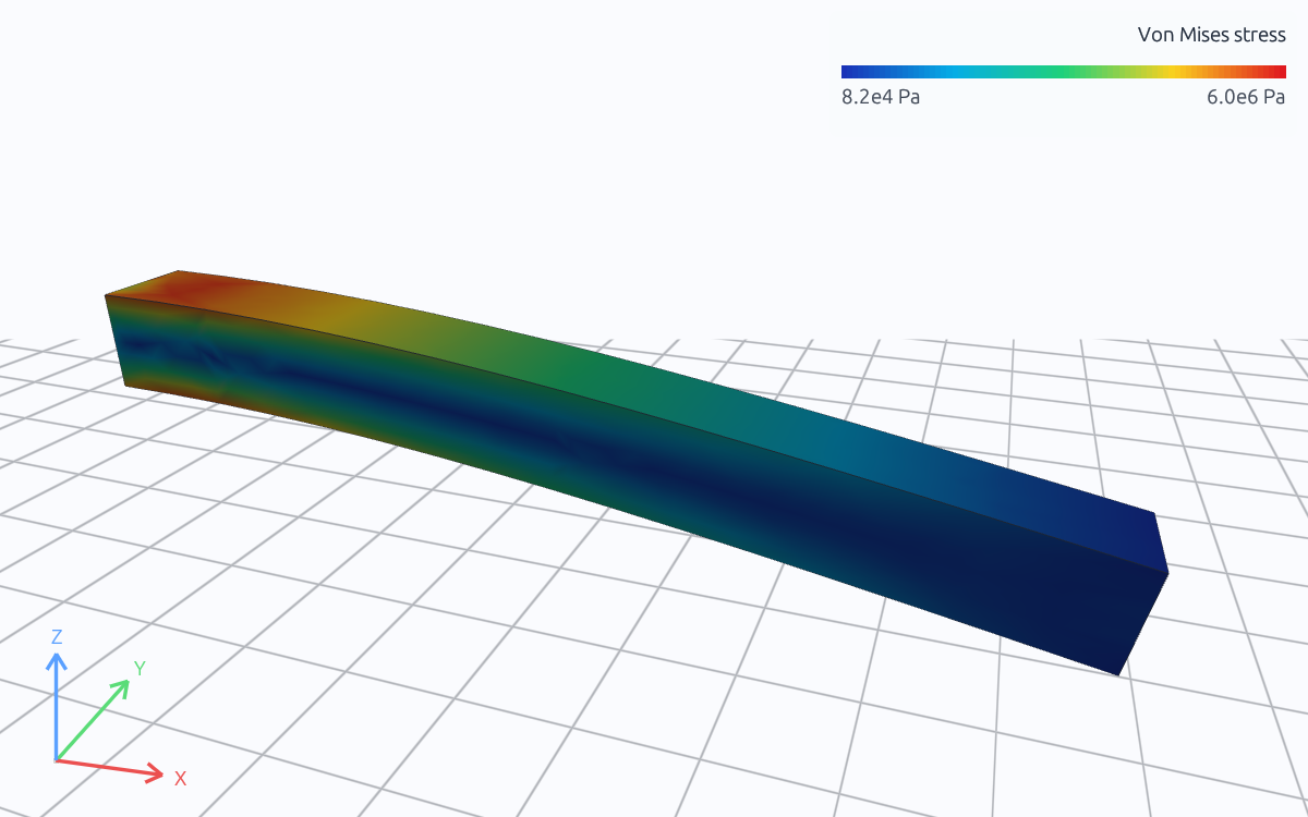
Von Mises stress · Pa · 8.25e+4 to 6.02e+6. Drag to rotate; scroll to zoom.
Color shows the element von Mises stress. As beam theory predicts, it is highest near the wall and on the top and bottom surfaces, and falls toward the free end.
The largest element value, 5.39 MPa, lies in an element on the fixed edge, and it is not a design value. Where a perfectly rigid face meets a free surface, linear elasticity predicts a stress singularity: the computed stress there keeps changing as the elements shrink, because no real support is perfectly rigid. A short distance from the wall the field is smooth. On the top surface at x = 100 mm the nodal von Mises stress is 5.43 MPa; beam theory gives M c / I = 5.4 MPa at the same section.
Answers
- Tip deflection: 0.2000 mm.
- Bending stress: 5.43 MPa on the top surface at x = 100 mm, rising toward about 6 MPa at the wall by the linear moment distribution.
- Wall reaction: 1,000 N upward and a moment of 1,000 N·m.
- The deflection is 40 % of the 0.5 mm limit, and the stress is under 4 % of the 167 MPa allowable. The beam meets both criteria.
Discussion
Design meaning. Both criteria pass, but by very different margins: the deflection uses 40 % of its limit, the stress under 4 %. The beam is governed by stiffness, which is typical of steel members sized to a deflection limit. A lighter section would reach the deflection limit long before the stress limit, so a redesign should keep and remove material where it contributes little to , for example by changing to an I-section.
Model limits. The analysis is linear: a 0.2 mm deflection on a 1 m span and a stress far below yield are well inside small-strain elasticity. The fixed face is an idealization. A real welded or bolted joint is somewhat flexible, which adds deflection at the tip and removes the singular peak at the edge. When the stress at the joint matters, model the joint itself: the weld fillet, the bolts, or the flexible support. The peak then becomes a real value that settles as the mesh is refined.
Refinement. A finite-element answer depends on the mesh, so the quantities a decision rests on should be checked on a finer mesh. Refining this beam from 150 mm to 50 mm changes the tip deflection by about 0.2 % and the stress at x = 100 mm by about 0.4 %, far less than the margins above. The mesh refinement guide works through the full sequence, and structural validation compares it with beam theory.
Try a change
Problem 1.1. Replace the steel with aluminum (youngs_modulus = 68.9 GPa). Predict the tip deflection and the stress at x = 100 mm before running. Does the beam still meet the deflection limit?
Answer. The deflection scales with 1/E, to about 0.2000 × 200 / 68.9 ≈ 0.58 mm, which exceeds the limit. The stress barely changes, because the moment at each section depends only on the load.
Problem 1.2. Double the load to 200 kPa. Because the problem is linear, deflection, stress and reactions all double; one solution covers every load level by scaling.
Problem 1.3. Change the mesh to linear tetrahedra (order = linear) at a 50 mm target size and compare the tip deflection with the Tet10 result. It falls well short, at 0.1625 mm: constant-strain elements cannot represent bending and make the beam too stiff.
Problem 1.4. Put the stress criterion in the study, so every run reports both verdicts. The two outputs run today; an assessment on a value sampled at a point is Not yet releasedStatus.
output top_stress = interpolate(analysis.static.field.node.von_mises_stress, at = [100 mm, 50 mm, 100 mm])
output support_reaction = resultant(analysis.static.field.node.reaction_force, over = geometry.beam.region.fixed_end)

assessment stress_allowable {
    value = output.top_stress
    maximum = 167 MPa
    evidence = authored_samples
}
Next
- Mesh refinement: a convergence study on this beam.
- Modal analysis: natural frequencies and mode shapes.
- Structural physics reference: every structural procedure and its equations.
- Structural validation: this beam against beam theory across mesh sizes.