
Finite-element analysis
Steady heat transfer
Prescribe end temperatures on a steel bar and explore its saved temperature and heat-flow fields.
Explore steady heat conduction
Hold one end of a steel bar at 300 K and the other at 350 K. RunMat solves for temperature inside the solid and recovers heat flux from its temperature gradient. The remaining surfaces have no applied heat flux.
Inspect the bar
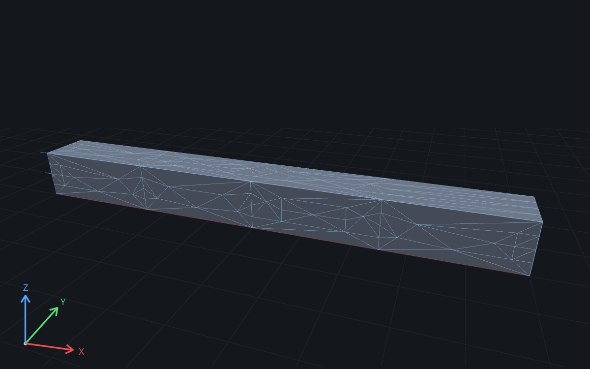
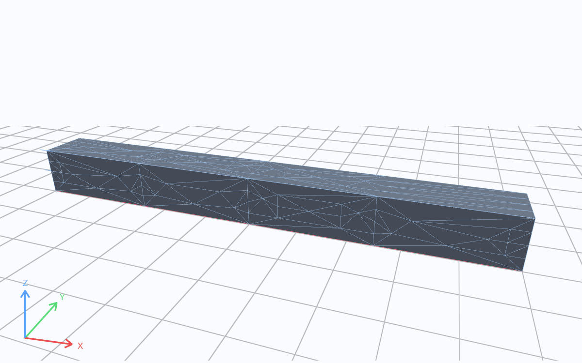
Solver mesh · m. Drag to rotate; scroll to zoom.
The study imports the cantilever STEP geometry and uses linear tetrahedra. Steel has a thermal conductivity of 45 W/(m·K). This model contains no volumetric heat source or convection boundary.
Inspect temperature
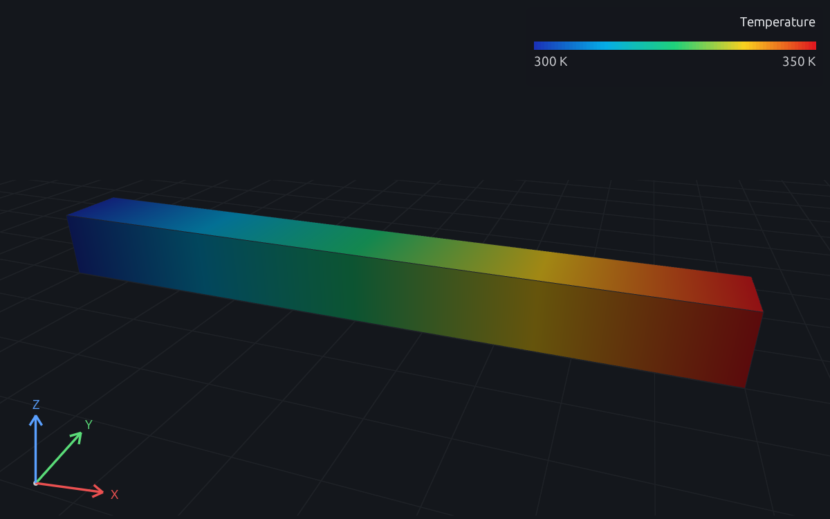
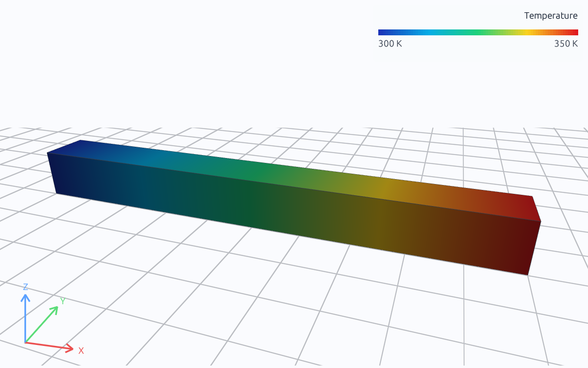
Temperature · K · 300 to 350. Drag to rotate; scroll to zoom.
Color shows temperature in kelvin. Compare the prescribed ends with the interior. Rotating or zooming the saved view does not repeat the solve.
Inspect heat flux
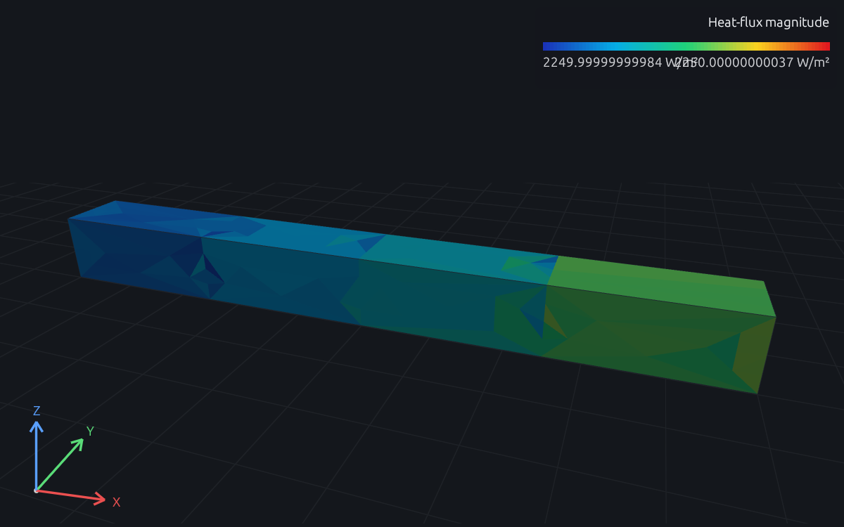
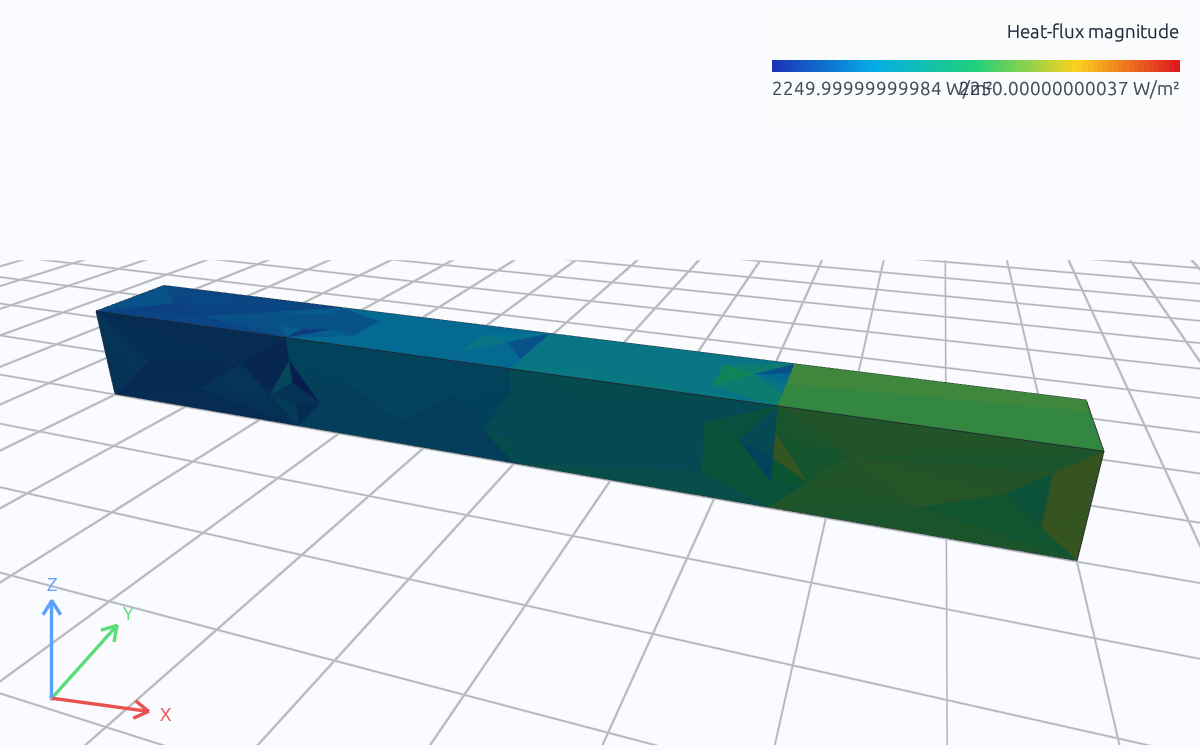
Heat-flux magnitude · W/m^2 · 2.25e+3 to 2.25e+3. Drag to rotate; scroll to zoom.
Color shows element heat-flux magnitude in W/m². The saved output retains the vector components. Heat flows from the hotter end toward the colder end.
Edit and run the study
Open the project in RunMat Desktop, or download it for the CLI. These excerpts come from the study source.
Import and mesh the bar
geometry beam {
    file = "./geometry/cantilever.step"
    units = mm
    region body : solid { select name "Beam"; expect exactly_one }
    region fixed_end : face { select name "Fixed end"; expect exactly_one }
    region loaded_end : face { select name "Loaded end"; expect exactly_one }
}

mesh beam on geometry.beam {
    tetrahedra {
        order = linear
        target_size = 1 m
        maximum_deviation = 0.001 m
    }
}
Set conductivity
material steel {
    mass_density = 7850 kg/m^3
    thermal {
        reference_temperature = 300 K
        modulus_temperature_coefficient = 0 K^-1
        expansion_coefficient = 0.000012 K^-1
        conductivity = 45 W/m/K
        specific_heat = 500 J/kg/K
    }
}
Prescribe end temperatures
model conducting_bar {
    thermal { reference_temperature = 300 K }
    assign material.steel to geometry.beam.region.body
    constraint cold_end {
        thermal.temperature { target = geometry.beam.region.fixed_end; value = 300 K }
    }
    constraint hot_end {
        thermal.temperature { target = geometry.beam.region.loaded_end; value = 350 K }
    }
}
Request fields
study conduction {
    geometry = geometry.beam
    mesh = mesh.beam
    model = model.conducting_bar
    analysis heat { thermal steady {} }
    output temperature = analysis.heat.field.node.temperature
    output heat_flux = analysis.heat.field.element.heat_flux
}Includes the study, STEP geometry, and saved results. Run new analyses in RunMat Desktop or the CLI.
View the complete study
// Engineering physics belongs in the importing study.

geometry beam {
    file = "./geometry/cantilever.step"
    units = mm
    region body : solid { select name "Beam"; expect exactly_one }
    region fixed_end : face { select name "Fixed end"; expect exactly_one }
    region loaded_end : face { select name "Loaded end"; expect exactly_one }
}

mesh beam on geometry.beam {
    tetrahedra {
        order = linear
        target_size = 1 m
        maximum_deviation = 0.001 m
    }
}

material steel {
    mass_density = 7850 kg/m^3
    thermal {
        reference_temperature = 300 K
        modulus_temperature_coefficient = 0 K^-1
        expansion_coefficient = 0.000012 K^-1
        conductivity = 45 W/m/K
        specific_heat = 500 J/kg/K
    }
}
model conducting_bar {
    thermal { reference_temperature = 300 K }
    assign material.steel to geometry.beam.region.body
    constraint cold_end {
        thermal.temperature { target = geometry.beam.region.fixed_end; value = 300 K }
    }
    constraint hot_end {
        thermal.temperature { target = geometry.beam.region.loaded_end; value = 350 K }
    }
}
study conduction {
    geometry = geometry.beam
    mesh = mesh.beam
    model = model.conducting_bar
    analysis heat { thermal steady {} }
    output temperature = analysis.heat.field.node.temperature
    output heat_flux = analysis.heat.field.element.heat_flux
}
From the project directory:
runmat check steady-conduction.fea
runmat plan steady-conduction.fea
runmat run steady-conduction.fea
Change either prescribed temperature or the conductivity, then solve again. The embedded figures retain the original example.
Model heater power and air cooling
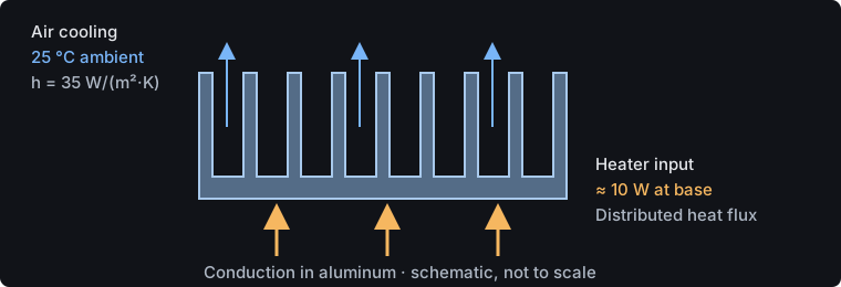
The downloadable heat-sink example imports a finned KiCad STEP model. A distributed heater supplies approximately 10 W to the mounting face. Aluminum with conductivity 160 W/(m·K) conducts heat into the fins, and a uniform film coefficient of 35 W/(m²·K) represents cooling to 25 °C air. Convection applies to the entire outer surface, including the heated mounting face. The example does not resolve airflow, a chip, a board or a thermal contact layer.
Try a complete example
Apply heater power to an aluminum heat sink and inspect conduction into its air-cooled fins.
Cool a finned electronics heat sink
Includes the study and its STEP assembly. Relative file paths are preserved.
Open or download the complete project, then run it in RunMat Desktop or the native CLI to compute temperature and heat flux.
Declared outputs
- Node temperature, in kelvin
- Element heat flux, in watts per square meter
View the complete study
// Engineering physics belongs in the importing study.

geometry heatsink {
    file = "./geometry/electronics-heatsink.step"
    units = mm
    region body : solid { select name "Heat sink"; expect exactly_one }
    region heater_face : face { select name "Mounting face"; expect exactly_one }
    region outer_surface : face { select result; expect one_or_more }
}
mesh heatsink on geometry.heatsink {
    tetrahedra {
        order = linear
        target_size = 10 mm
        maximum_deviation = 0.1 mm
    }
}
material aluminum {
    mass_density = 2700 kg/m^3
    thermal {
        reference_temperature = 298.15 K
        modulus_temperature_coefficient = 0 K^-1
        expansion_coefficient = 0.000023 K^-1
        conductivity = 160 W/m/K
        specific_heat = 900 J/kg/K
    }
}
model cooled_heatsink {
    thermal { reference_temperature = 298.15 K }
    assign material.aluminum to geometry.heatsink.region.body
    load heater {
        thermal.heat_flux {
            target = geometry.heatsink.region.heater_face
            value = 2290.319 W/m^2
        }
    }
    load air_cooling {
        thermal.convection {
            target = geometry.heatsink.region.outer_surface
            ambient_temperature = 298.15 K
            coefficient = 35 W/m^2/K
        }
    }
}
study heatsink_temperature {
    geometry = geometry.heatsink
    mesh = mesh.heatsink
    model = model.cooled_heatsink
    analysis heat { thermal steady {} }
    output temperature = analysis.heat.field.node.temperature
    output heat_flux = analysis.heat.field.element.heat_flux
    output peak_temperature = max(analysis.heat.field.node.temperature, over = geometry.heatsink.region.body)
    assessment stays_below_85_celsius {
        value = output.peak_temperature
        maximum = 358.15 K
        evidence = authored_samples
    }
}
This project includes the geometry and its original license. Run it in a native Desktop or CLI installation to compute its fields. No saved heat-sink result is included in this guide.
Thermal formulation
Steady conduction satisfies
Conductivity relates the temperature gradient to heat flux . Volumetric generation supplies heat inside a solid. The bar sets and prescribes end temperatures. For convection, outward heat loss is .
RunMat integrates the solid and boundary terms, solves for nodal temperature, and recovers element heat flux. Choose a transient study when heat capacity and warm-up or cool-down matter.
See thermal validation for formulation and recovery checks, and thermal loads for temperature, power and convection boundaries.